Reduced Step Point Collocation Interpolation Method for the Solution of Heat Equation

In this study, we developed a new finite difference approximate method for solving heat equations. We study the numerical accuracy of the method. Detailed numerical results have shown that the method provides better results than the known explicit finite difference method. There is no semidiscretization involved and no reduction of PDE to a system of ODEs in the new approach, but rather a system of algebraic equations directly results.

Keywords: Lines; Multistep collocation; Parabolic; Taylor’s polynomial

In this study, we will deal with a single parabolic partial differential equation in one space variable, where and are the time and space coordinates respectively, and the quantities and are the mesh sizes in the space and time directions. we consider,, 0 ≤ x ≤ b, 0 ≤ t ≤ T ………. (1)

Subject to the initial and boundary conditions

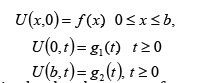
We are interested in the development of numerical techniques for solving heat equations. Of recent, there is a growing interest concerning continuous numerical methods of solution for ODEs [1- 3]. We are interested in the extension of a continuous method to solve the heat equation. This is done based on the collocation and interpolation of the PDE directly over multi steps along lines but without reduction to a system of ODEs. We intend to avoid the cost of solving a large system of coupled ODEs often arising from the reduction method by semi-discretization. The method also, eliminates the usual draw-back of stiffness arising in the conventional reduction method by semi-discretization [4,5].

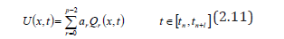
We subdivide the interval 0 ≤ x ≤ b into N equal subintervals by the grid points x_m = mh, m =0,..., N where Nh = b .On these meshes we seek l − step approximate solution to U(x,t) of the form

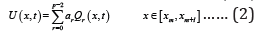
such that The basis function Q_r(x,t),r= 0,..., p − 2 are assumed known, a_r are constants to be determinedand p ≤ l + s , where s is the number of collocation points. The equality holds if the number of interpolation points used is equal to l . There will be flexibility in the choice of the basis function Q_r(x t), as may be desired for specific application. For this work, we consider the Taylor’s polynomial . The interpolation values are assumed to have been determined from previous steps, while the method seeks to obtain , [1,2,6,7]. We apply the above interpolation conditions on eqn. (2) to obtain

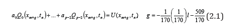
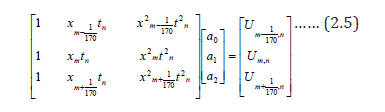
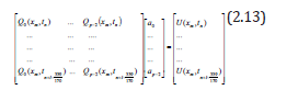
We can write eqn. (2.1) as a simple matrix equation in the augmented form as,

Using three interpolation points and one collocation point, implies that s =1, p = 4, l = 3 and r = 0,1,2.

Substituting for p in eqn. (2.1) we have,

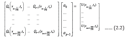
Putting the values of g in eqn. (2.3) and writing it as matrix in augmented form
we have,

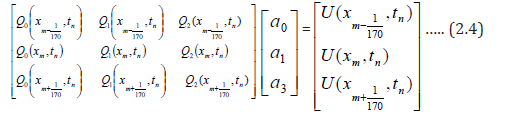
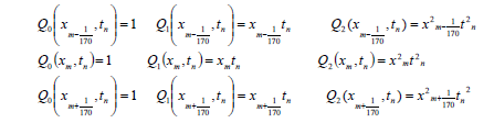
From eqn. (2.4) we obtain the following values

Putting the above values in eqn. (2.4) becomes

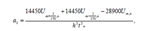
When we solve eqn. (2.5) to obtain the value of a₂ to be

We substitute r = 0,1,2 in eqn. (2.0) to obtain

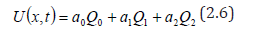
By substitution of Q₀ Q₁ and Q₂ in eqn. (2.6) we obtain

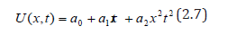
Substituting the value of a₂ in eqn. (2.7) we obtain

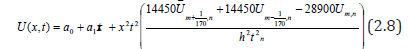
Taken the first and second derivatives of eqn. (2.8) with respect to we have

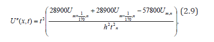
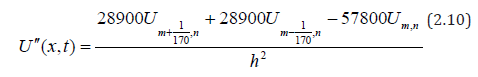
we collocate eqn. (2.9) at t = t_n to arrive at

Similarly, we reverse the roles of x and t in eqn. (2.0), and we also subdivide the interval 0 ≤ t ≤ T into y equal subintervals by the grid points 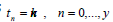where yk = T. On these meshes we seek l − step approximate solution to U(x,t) of the form

Such that 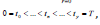, the basis function 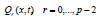are assumed known, a_r are constants to be determined and p ≤ l + s , where s is the number of collocation points. The equality holds if the number of interpolation points used is equal to l . There will be flexibility in the choice of the basis function Q_r(x t), as may be desired for specific application. For this method, we consider the Taylor’s polynomial .The interpolation values are assumed to have been determined from previous steps, while the method seeks to obtain [see (4)]. We apply the above interpolation conditions on eqn. (2.11) to obtain

We can write (2.12) as a simple matrix equation in the augmented form

Using two interpolation points and one collocation point in eqn. (2.13) implies that p = 3, r = 0,1 l = 2 and , and by substitution eqn. (2.13) becomes

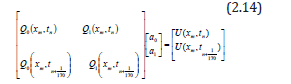
From eqn. (2.14) we obtain the following values:

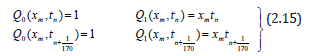
Substituting the values of eqn. (2.15) into eqn. (2.14), we have this matrix below

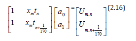
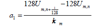
Solving eqn. (2.16) for value of a₁ we obtain

When we substitute r = 0,1, into eqn. (2.11), we obtain

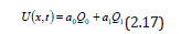
By substituting the values of in equation (2.17) we have

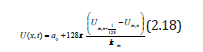
Taken the first derivatives of equation (2.18) with respect to t we obtain

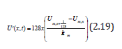
We collocate eqn. (2.19) at x = x_m yields

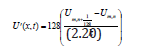
But from eqn. (1.0) we find that eqn. (2.20) is equal to eqn. (2.10), which implies that

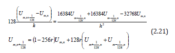
manipulating mathematically and putting , we obtain Eqn. (2.21) is a new scheme for solving the heat equation. To illustrate this method, we use it to solve problems (3.1) and (3.2) respectively.

1.1. Advantages of the method
A. We intend to avoid the cost of solving a large system of coupled ODEs often arising from the reduction methods.
B. We also intend to eliminate the usual draw-back of stiffness arising in the conventional reduction method by semi-discretization.

Example

Use the scheme to approximate the solution to the heat equation (Table 1)

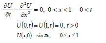
Table 1:Result of action of Eqn. (2.21) on problem 3.1.

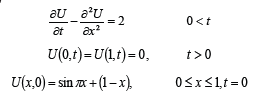
Example

Table 2:Result of action of Eqn. (2.21) on problem 3.2.

Use the scheme to approximate the solution to the heat equation (Table 2)

A continuous inter-polant is proposed for solving parabolic partial differential equation in one space variable without discretization. To check the numerical method, it is applied to solve two different test problems with known exact solutions. The numerical results confirm the validity of the new numerical scheme and suggested that it is an interesting and viable numerical method which does not involve the reduction of PDE to a system of PDE to a system of ODEs.

1. Odekunle MR (2008) Solution of partial differential equation using collocation interpolation method.
2. Pierre J (2008) Numerical solution of the dirichlet problem for elliptic parabolic equations. SIAM J Soc Indust Appl Math 6(3): 458-466.
3. Ang WT (2006) Numerical solution of a non-classical parabolic problem: an integro-differential approach. Appl Math Comput 175(2): 969-979.
4. Bensoussan A, Da Prato, Delfour GM, Mitter S (2007) Representation and control of infinite dimensional systems (2^nd Edn), Systems & Control: Foundations & Applications, Springer, Berlin, Germany.
5. Jain MK (1991) Numerical solution of differential equation. Wiley Eastern limited, New Delhi, India.
6. Odekunle MR (2006) Solutions of linear evolutionary equations using lanczos-chebyshev reduction. Global Journal of Mathematics Science 5(2).
7. Odekunle MR (2008) Solution of partial differential equation using collocation interpolation method. A conjecture. Paper presented at the annual conference of the Nigeria Mathematical Society, University of Lagos, Lagos, Nigeria.