Adsorption Isotherm Deduced from the Billiard Model and Equation of State of a Gas of Interacting Soft Spheres

Introduction

Several equations of state have been proposed to describe the thermodynamic behavior of real gases. The equation of state of ideal gases deduced by combining the Gay-Lussac and Boyle-Mariotte laws was modified by van der Waals in order to take into account the attraction between molecules and their finite volume. His equation predicted the critical point of real gases. After division of the temperature T, pressure p, and molar volume V_m by their critical values, the van der Waals equation reduces to a single expression of the reduced variables

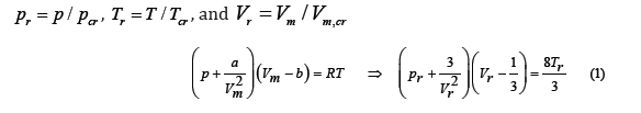
where the constants a and b are related to the critical parameters [1] through

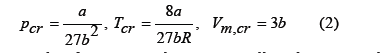
which implies the principle of corresponding states: all real gases at the same reduced temperature and pressure have the same compressibility factor (or have the same reduced volume). At the critical point, the van der Waals equation predicts a compressibility factor , p_cr V_m, _cr/ (RT_cr) =0.375 , although for most gases its value is slightly less than 0.3. The principle of corresponding states, although an approximation, is more accurate than the van der Waals equation, so that graphs of reduced thermodynamic variables that are general for all gases can be drawn from experimental data, even though they separate from the van der Waals equation. One of our goals is to find an algebraic equation of state for real gases able to fit well the graph of the compressibility factor as function of the reduced temperature and pressure.

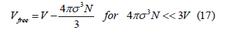
Van der Waals assumed that the exclusion volume is proportional to the number of moles n, and that the free volume is V_free =V − nb , where the covolume b is a constant characteristic of each gas, which is higher than the molar volume in the solid state and approximately four times the volume of the molecules according to him [2,3]. This simplified assumption differs from the observed behavior of real gases because the free volume of a gas of hard spheres depends on the density not linearly as van der Waals assumed, but in a more complex way. In fact, the exclusion volume depends not only on density but also on temperature. Both elements will be discussed below.

For two dimensions, several adsorption isotherms were proposed to describe the adsorption of ions and neutral compounds. Damaskin et al. [4] listed up to 14 different isotherms. The most widely used are the Langmuir, Frumkin and virial isotherms. Langmuir [5] deduced his isotherm

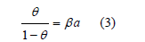
under the hypothesis that molecules absorb localized sites of the surface. 𝜃 is the coverage, 𝛽 is the adsorption coefficient (a constant), and a is the activity, which is proportional to pressure at constant temperature for dilute gases, that is, 𝛽 only depends on the temperature. He verified his isotherm with the adsorption of several gases (N2, CH4, CO, Ar, O2, and CO2) on mica at 155K and on glass at 90K. However, adsorption from aqueous solutions was first measured at room temperature and on the dropping mercury electrode, for which localized adsorption sites are meaningless because the electrode is liquid. The Langmuir isotherm, like the van der Waals equation, also considers an exclusion area proportional to the coverage. Frumkin [6] introduced an attractive term into the Langmuir isotherm analogous to that in the van der Waals equation

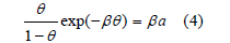
where the constant B plays the same role as (it is twice) the van der Waals’ constant a in (1). As Frumkin himself showed, his isotherm also predicts phase transitions for values of B>4 [6], and the critical point at B=4. In the virial isotherm, the logarithm of the activity is equal to the logarithm of the surface excess 𝛤 plus a virial expansion in powers of 𝛤, of which only the second virial coefficient is usually taken into account: ln Γ + BΓ = lnβ + ln a [7]. This isotherm does not have maximum surface excess, so that it avoids the problem of its determination. We faced [8] the problem of the maximum surface excess or the maximum adsorption charge when we tried to reproduce the adsorption of halides by means of a Frumkin isotherm modified for ionic adsorption

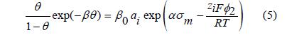
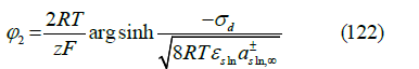
where β₀ is the adsorption coefficient at zero metal charge, a_i is the ionic activity of the ion i in the solution, φ₂ is the diffuse layer potential drop (the difference of electric potential between the boundary of the diffuse layer and the bulk solution), z_i is the charge number of the adsorbed ion, F is the Faraday constant, R is the gas constant, σ _m is the metal (electrode) charge and α is a constant that accounts for the experimental observation that ln β depends linearly on the metal chargeσ _m . As explained in [9] and reviewed below in the section on the ionic adsorption isotherm, the argument of the exponential function is thermodynamically consistent with an electric potential drop across the interface described by a capacitor of three plates, namely: the metal surface, the inner Helmholtz plane (IHP) containing the centers of the specifically adsorbed ions, and the outer Helmholtz plane (OHP) which is the boundary of the diffuse layer. The electric polarization in the diffuse layer is usually described by the Gouy-Chapman theory, and the polarization between the IHP and the OHP is modeled as a linear dielectric medium whose permittivity is proportional to α .

We reproduced successfully [8] the curves of electric capacity versus metal charge for halide adsorption on mercury, but at the cost of unrealistic maximum adsorption charges¹: for chloride and iodide, with B=0 for chloride and B=-7.16 for iodide. The adsorption charges calculated from the ionic radii for a close-packed hexagonal lattice are for chloride and for iodide. At that time (in 1989), this paradox remained unsolved until we realized, after playing a billiard game with a friend, that halide adsorption could be well described by the billiard model [10]. The very negative value of Frumkin’s interaction parameter of iodide was also explained by the dielectric saturation of the zone between the IHP and the OHP.

Free-area function in the billiard model

Since halide ions have closed electronic shells and are spherical, and their specific adsorption was firstly

studied on the dropping mercury electrode, which is liquid and has no structured surface, we thought that their adsorption on metal electrodes could be modeled as billiard balls on a table. The billiard model is nothing more than a visual representation of a two-dimensional gas of hard spheres. We tested [10] the adsorption isotherm deduced from the billiard model with halide adsorption, obtaining a good result for chloride and not so good for iodide. Details are given below in the section on the ionic adsorption isotherm.

¹ Coverage was calculated as , where σ₁ is the specific adsorption charge of the anion since the cation is assumed not to be specifically adsorbed.

In the billiard model, there are no specific locations, and every point on the surface is available to a ball unless it belongs to the exclusion circle of another ball. The balls move freely on the surface except in collisions with other balls. The balls are hard spheres having a radius R. The balls in their motion are represented by their centers as in classical physics. The free-area function of a surface partially covered by a certain amount of balls is defined as the fraction of surface area available for the center of a new ball to adsorb. Let us imagine that there is only one ball on the surface. Since the center of two balls cannot be closer than 2R (Figure 1), the exclusion area occupied by a ball is exactly 4π R² , four times the area of the ball’s projection onto the surface. Therefore, at low coverage when intersections between the exclusion circles can be disregarded, the free-area function has the approximate linear expression

Figure 1:The centers of two spheres cannot approach each other at a distance less than their diameter.

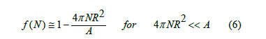
where N is the number of balls on the surface, and A is the total area of the surface.

The free-area function depends on N, but it is better to use a molar fraction as independent variable. Although the projection area of a ball is π R² , the cell area of a close-packed hexagonal lattice of balls on a surface is slightly larger, 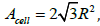, due to interstitial spaces. Therefore, the maximum surface excess of hard balls in a close-packed lattice is

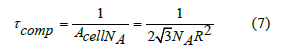
where N_A is the Avogrado constant. We define the coverage as the ratio of balls on the surface to the number of balls in a closepacked hexagonal lattice

The empty surface has zero coverage and the close-packed lattice of balls has unit coverage. Therefore, the linear approximation to the free-area function as function of coverage is

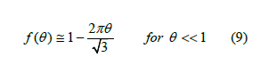
What happens when coverage increases? Intersections between the exclusion circles with radius 2R become more frequent and the linear law no longer holds. There is not an easy way to calculate the area of these intersections. Thus, we resorted to simulations to determine the free-area function (details below). The result of averaging many simulations was a curve that can be quite well fitted by a quadratic function. The parameters of this fit depends on each set of simulations, so we proposed as a theoretical approximation a quadratic function that satisfies (9) and is tangent to the abscissa axis²

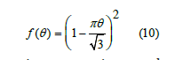
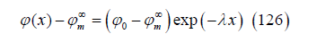
This quadratic function overestimates the true free area, as shown in Figure, and reduces to zero at a maximum coverage less than unity

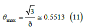
Simulations indicate that the free area becomes zero on average for coverage values slightly greater than 0.57. With the billiard isotherm, the interface reaches saturation around this coverage, but higher coverages are possible for balls in a lattice, which are described by the Langmuir isotherm. For halide ions, the phase transition between delocalized adsorption and localized adsorption is reproduced by both isotherms at coverages that are close to the maximum coverage (11) and depend on the halide masses, because the translational entropy of the billiard isotherm is much higher than the configurational entropy of the Langmuir isotherm. This phase transition occurs experimentally, and ordered configurations of halide ions on crystalline surfaces are only observed [11] at adsorption charges higher than −0.96C.m⁻² (θ = 0.68) for chloride, −0.74C.m⁻² (θ = 0.62) for bromide, and −0.34C.m⁻² (θ = 0.32) for iodide, although the thresholds depend on the nature and crystalline face of each electrode.

Simulations were carried out to obtain the free-area function. In a unit-sided square on the computer screen, the centers of the exclusion circles are randomly placed following a two-dimensional uniform distribution with the only condition that they cannot be closer than 𝜎=2R (Figure 2). If the coordinates of a new center do not satisfy this condition, they are discarded and new random coordinates are calculated. After validating the center, its exclusion circle of radius 𝜎=0.1 is painted, and the unpainted pixels of the square are counted to obtain the free-area function. In this way, the surface is progressively covered until the free area is exhausted. The free-area function is the ratio of unpainted pixels to scanned pixels, which are a sample of pixels on a grid. More details can be found in [8]. The random boundary conditions were taken as follows: the exclusion circles with centers in the square [0,1]² are painted, but the free-area function is calculated by scanning only the square [𝜎,1-𝜎]², and the coverage is calculated by counting only the circles whose centers are inside this latter square. In this way, other balls randomly surround the counted balls on all sides. In [8], we incorrectly scanned the square [R, 1-R]², which is too large and has too small random boundary because the exclusion circles have radius 𝜎=2R. The boundary conditions were then corrected in [12] by scanning only the square [𝜎, 1-𝜎]².

² Disordered ball configurations with coverage greater than 0.58 are unlikely but not impossible, so the free area function approaches the abscissa axis asymptotically. Therefore, it is not acceptable for a free-area function to reach the abscissa axis at a certain angle.

Figure shows the free-area function obtained by averaging 100 simulations compared to the theoretical quadratic function (10), which overestimates the free area and predicts a maximum coverage of 0.5513, slightly lower than 0.57 observed in the simulations. More details can be found in [10,12]. In molecular dynamics studies, the free-area function is also known as the available surface function [13,14] (Figures 2-4).

Figure 2:Halfway through the simulation. Exclusion circles in green, and free area in black.

Figure 3:Cell of a close-packed hexagonal lattice of hard spheres. In gray the shadow of the sphere in this cell.

Figure 4:Intersection of two exclusion circles or spheres of radius σ whose centers are separated by a distance r. The intersection is twice the circular segment or spherical cap with height h =σ − r / 2 .

Equation of state and adsorption isotherm of a gas of hard spheres

In this section, the equation of state of a hard-sphere gas will be derived simultaneously for two and three dimensions. d will denote dimension, V_d will denote area or volume (V₂=A, V₃=V), p will denote either the surface pressure γ₀ −γ (γ is the surface tension) or pressure of a volume of gas. For two dimensions, the cell area of a close-packed hexagonal lattice is and the coverage is defined by (8). We also define the shadow 𝜙, which is proportional to the coverage, as

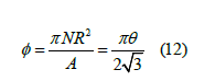
If we hang a lamp over the billiard table, the shadow is the fraction of the area shaded by billiard balls relative to the total area of the table (Figure 3). The shadow can vary in the interval 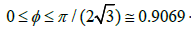. When the billiard table is filled with a close-packed hexagonal lattice of balls, approximately 10% of the surface is still illuminated. It will be seen that the shadow is a better variable for the deduction that follows. For example, the free-area function (10) becomes

In three dimensions, there are two compact arrangements of hard spheres: the hexagonal lattice and the face-centered cubic lattice. Both lattices have the same density. The volume of the rhombohedral cell containing a sphere of radius R is

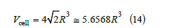
This volume is larger than the volume of a sphere 4π R³ / 3 ≅ 4.1888R³ because of the interstitial holes. We define the filling ψ as the ratio of the number of spheres in a given volume to the number of spheres in a compact lattice

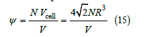
The filling is a molar fraction ( 0 ≤ψ ≤1). A widely used variable in the hard-sphere gas literature that is similar to shadow is the packing fraction

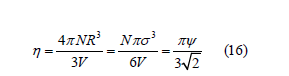
which is proportional to the filling. The packing fraction ranges as . It is a better variable for the deduction that follows.

The free volume is defined as the volume available to the center of a new sphere when the volume already contains other spheres. Let us consider that there is only one sphere in the volume. The exclusion volume is the volume where the center of a new sphere cannot be placed. Since the centers of two spheres cannot approach closer than a distance 𝜎=2R, the exclusion volume of one sphere is 4𝜋𝜎³/3 Therefore, when the density is low, the free volume approximately follows the linear law

The free-volume function is defined as the ratio of the free volume to the total volume

At middle and high densities, the free-volume function no longer fits this linear approximation. Its determination is explained below in the section on the determination of the free-volume function.

Let us now derive the equation of state of a gas of hard spheres in d dimensions (two or three). The translational canonical partition function of a particle i in a box with d -volume V_d [10, Equation 17], [15, Equation 4.23] is

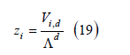
where is the thermal wavelength (h is the Planck constant, m is the mass of the particle, k is the Boltzmann constant and T is the absolute temperature), and V_id is the free d -volume available for the sphere i to be added to the system. Adding more spheres progressively reduces the free d -volume according to 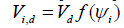where ψ_i is the filling for i spheres in the system ( ψ_i can also be replaced by θ_i because the deduction is general). Therefore, the total translational canonical partition function of a system of N spheres within a d -volume V_d is

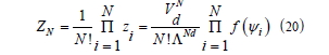
where Gibbs’ correction for undistinguishable particles has been taken into account. Taking logarithms, using the Stirling approximation and approximating the sum by an integral give

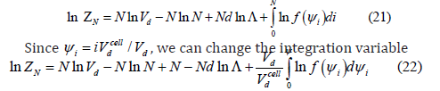
where 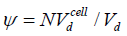is the filling or the coverage. Then, the free Helmholtz energy is

In two dimensions, the adsorption energy Nu, where u is the adsorption energy of a molecule, can be added to F, but this does not change the surface pressure or the isotherm, since u is a constant added to the chemical potential that is included in the adsorption coefficient 𝛽 in (35). The pressure is obtained as the negative derivative of the Helmholtz free energy with respect to the d -volume at constant temperature and number of particles

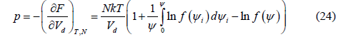
This equation is the same as [16, Equation 2].
After integration by parts, the compressibility factor becomes

The virial expansion of the compressibility factor is usually given in terms of the packing fraction

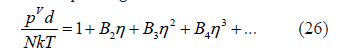
The identification of (25) and (26) allows us to obtain the free- d -volume function from the virial coefficients by isolation, differentiation and integration

whose expansion up to second order is

If a power law is fitted to the free- d -volume function, it must be of the form

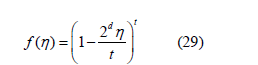
because of the linear approximations (9) (equivalent to f (φ ) ≅ 1− 4φ ) and (18) at low filling

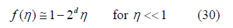
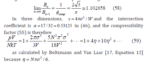
Where 𝜂 can be replaced by 𝜙. For d = 3, Boltzmann calculated the free-volume function [17, Equation 11]

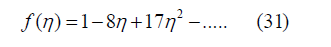
and therefore, the third virial coefficient as B₃ = 10 [18] since B₂ = 4. The later bibliography confirmed this calculation [19,20]. However, we obtained an exponent t = 3.2 in (29) from three-dimensional simulations [12], which corresponds to f (η ) =1−8n + 22η ² −..... and B₃ = 20/3. This discrepancy with Boltzmann’s result helped us to realize that the boundary conditions in our simulation were taken incorrectly. They have been corrected here, which is explained below in the section on the determination of the free-volume function. The equation of state obtained from the power law (29) by means of (25) is

For the free-area function given by the quadratic law (13), t = 2 and d = 2, so the surface pressure p (the difference γ₀ −γ between the surface tension in the absence and presence of adsorption) is

On the other hand, the chemical potential is obtained as

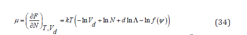
Taking into account that ln ln ln cell ln 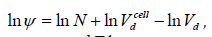and expressing the chemical potential μ = μ₀ + kT ln a as function of the activity a, we obtain

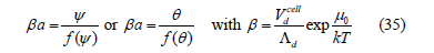
which is the adsorption isotherm in two dimensions but also held in three dimensions. 𝛽 is a constant (in two dimensions it is called the adsorption coefficient) that depends only on temperature but not on filling or coverage. Due to the equality of chemical potentials between the adsorption phase and the solution, a is the activity in the solution. This formalism assumes that the interface is empty and only one compound is adsorbed. If two compounds are assumed to coadsorb, the formalism is different and the chemical potentials in the solution are no longer equal to the interfacial chemical potentials. In this case, the Randles relations [21] involving surface tension must be applied as explained in [9]. In salt solutions, the adsorption layer contains solvent molecules, but the one-compound formalism is still valid because the solvent molecules are easily displaced by the adsorbed ions as if the adsorption layer were empty. In this case, the observed adsorption coefficient is only apparent and depends on the solvent. The coadsorption and apparent adsorption isotherms were discussed in [9].

Third virial coefficient of a hard-sphere gas

The second virial coefficient B₂ is related to the free d –volume available to a second sphere when a first sphere is already present in the system. In fact, B₂ is proportional to the exclusion d -volume of a sphere [15, p. 388]. This yields the linear law (30). The third virial coefficient is related to the free d -volume available to a third spherical particle when two of them are already present in the system. Depending on the positions of both particles, their exclusion d -spheres may intersect increasing the free d -volume available to the third particle.

In two dimensions, the area of the overlap of two exclusion circles of radius σ whose centers are separated by a distance r is twice the area of the circular segment (Figure 4)

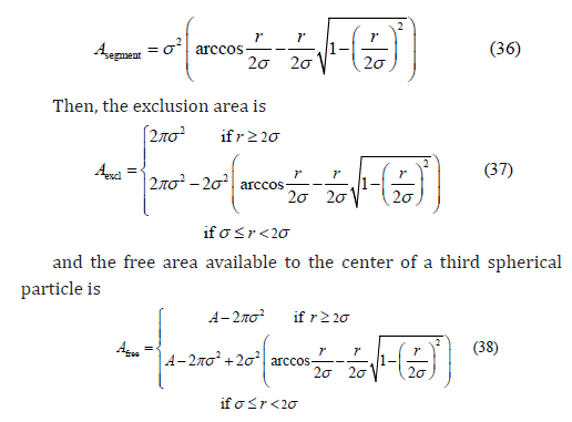
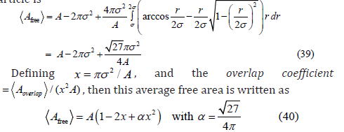
If the relative Cartesian coordinates of both particles follow a two-dimensional uniform distribution, then the radial distribution is given by 2π r dr / A , and the average free area available to a third particle is

Let us consider the three-dimensional case. When two exclusion spheres partially intersect, the volume of the intersection is twice the volume of the spherical cap (Figure 4)

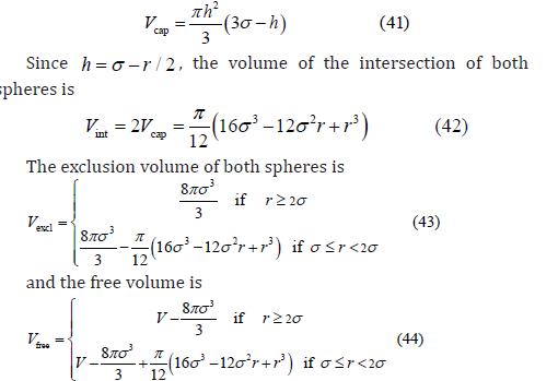
If the relative Cartesian coordinates of both particles follow a three-dimensional uniform distribution, then the radial distribution is given by 4π r² dr /V , and the average free volume available to the center of the third spherical particle is

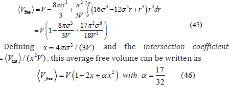
The average free area (40) and free volume (46) have the same expression so that the derivation of the third virial coefficient is the same for both dimensions. Then, the canonical partition functions of each particle are

The expansion of the logarithm of the grand partition function to third order gives

The coefficients of the powers of a in this expansion are

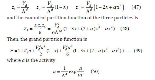
If the pressure is expanded in powers of the concentration ρ = N /V_d , then the virial coefficients are related with the previous coefficients by [15, Equation 11.37]

because x <<<1.

A list of several virial coefficients B_{n, p} for a two-dimensional gas of hard spheres (also called hard disks) calculated in different works was given in [23, Table 1] as the quotients 1 . Since , the dimensionless virial coefficients are obtained from these quotients by means of 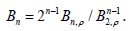. The results to six decimals places are shown in Table 1.

Table 1:Virial coefficients for a two-dimensional gas of hard spheres.

The quotients of consecutive coefficients B_n /B_n−1 tend to the inverse of the convergence radius of the virial series that should diverge at the shadow of a close-packed hexagonal lattice

Improvement of the polynomial approximation to the free-area function

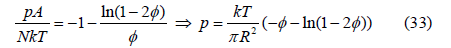
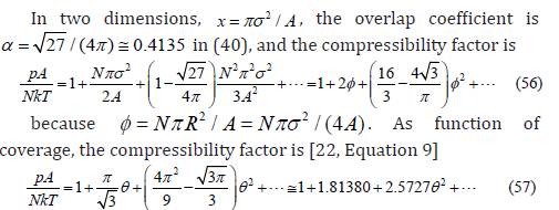
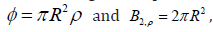
The expansion of the logarithm in the surface pressure (33)

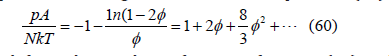
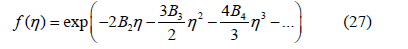
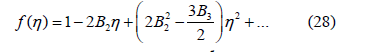
obtained from the quadratic free-area function (13) yields a third virial coefficient B₃ = 8 / 3 ≅ 2.6667 , but the third virial coefficient actually is B₃ ≅ 3.1280 as calculated in (56) and shown in Table 1, so the approximation to the free-area function needs to be improved as shown in Figure 5. Two different functions can be proposed: a cubic polynomial and a power law. Each curve must be tangent to the abscissa axis. The free-area function obtained from the virial coefficients by expansion of the exponential in (27) to third order is

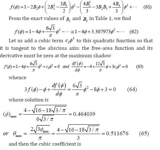
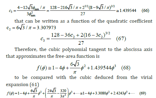
calculated with the known exact value of the fourth virial coefficient [24] listed in Table 1. The function (69) does not touch the abscissa axis, so it needs a fourth-order term to reach zero value. We believe that the cubic approximation (68) is good enough for applied and technical purposes. It can also be written as function of coverage

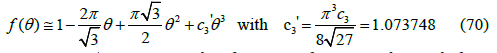
Figure 5 compares the free-area function obtained from simulations (squares) with the cubic function (70) that already includes the third virial coefficient, and with the quadratic function (13). The cubic function (middle line) fits simulations better than the quadratic function (upper line) but still differs slightly from them as shown in Figure 6. On the other hand, the maximum coverage (65) predicted by the cubic ( θ_max ≅ 0.5117 , φ_max ≅ 0.4640) is smaller than that predicted by the quadratic function ( θ_max = 3 /π ≅ 0.5513 ,φ_max =1/ 2 ), which is also smaller than observed in simulations ( θ_max ≈ 0.57 ). The adsorption isotherm (35) is therefore

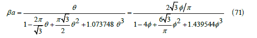
Figure 5:Free-area function obtained from averaging 100 simulations (squares) compared with the quadratic function (13) (upper curve), the cubic function (70) (middle curve), and the power law (72) (lower curve).

Figure 6:Free-area function obtained from averaging 100 simulations (squares) against the cubic (70) for the same coverage. The free-area function is slightly lower than the cubic at middle coverage but higher at saturation where a maximum coverage higher than predicted by the cubic can be reached. The line with unity slope is the identity.

The Langmuir isotherm and the quadratic and cubic approximations to the billiard isotherm isotherms are plotted in Figure 7 together with their maximum coverage.

Figure 7:Coverage against the reduced activity for (from top to bottom) the Langmuir isotherm (3), the quadratic (10) and cubic (70) billiard isotherms together with their respective maximum coverage (horizontal lines).

Another option for the free-area function is the power law

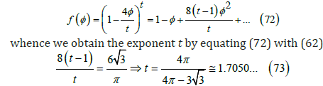
This exponent is less than 2 in the quadratic approximation (13). The maximum coverage predicted in this case is θ_max ≅ 0.4700 or φ_max = t / 4 ≅ 0.4263 . Figure 5 shows that it differs from simulations close to the maximum coverage, and that the cubic function is better.

Determination of the free-volume function

Simulations were carried out [12] to find the free-volume function by placing spheres randomly within a unit cube, checking that their centers are no closer tan 𝜎, scanning this volume and counting the points located outside all the exclusion spheres. The free-volume function is the probability of any point to be available for the center of a new sphere to be added to this volume [16]. Therefore, it is not necessary to scan points in the entire volume. Instead, points in a subset like a plane or even a line can be scanned. All three options were programmed [12] resulting in similar freevolume functions but with different deviations from the mean. Scanning the entire cube is very slow. Scanning a transversal plane is faster, and deviations are not very large. Scanning a line is very fast but deviations are much larger, so that means having significant errors according to the central limit theorem. Scanning a transversal plane seemed to be the optimal algorithm. The function that best fitted the simulations was the power law (29) with the exponent 3.2, which predicts a free-volume function f (η ) =1−8η + 22η ² −.... and a third virial coefficient B₃ = 20/3. However, Van Laar found f (η ) =1−8η +17η ² −.... [17, Equation 11] and Boltzmann found B₃ = 10 [18]. We also recalculated the third virial coefficient by three different analytic ways always obtaining Boltzmann’s result B₃ = 10 (one way using the grand partition function is explained above in the section on the third virial coefficient of a hard-sphere gas and leads to the virial expansion (59). To resolve this contradiction, we reexamined our simulations, and we realized that the boundary conditions were incorrect. After taking the correct boundary conditions, the agreement between the simulations and the freevolume function obtained from (27) using all the virial coefficients given in the bibliography up to B₁₂ is excellent as shown in Figure 8.

Figure 8:Free-volume function obtained by averaging 100 simulations (squares) against that calculated from (27) with the virial coefficients up to B₁₂ given in [25]. The line is the identity.

Let us explain why these boundary conditions of the twodimensional counting were wrong. In [12], the centers of the exclusion spheres of radius 𝜎 = 2R = 0.1 were randomly distributed in the box [0,1]² ×[−σ ,σ ] according to a three-dimensional uniform distribution always ensuring that the distances between them were greater than 𝜎. At the same time, the exclusion circles that are intersections of the exclusion spheres with the plane z = 0 were painted in the square [0,1]² on the screen. That is, z is the coordinate perpendicular to the computer screen, and z = 0 is the plane of the screen. If a center of a sphere has coordinates (x, y, z), then the exclusion circle with center (x, y) and radius is painted in the square. At each step of the simulation, the square [σ ,1−σ ]² is scanned, and the ratio of unpainted points to the scanned points gives the free-volume function. The scanned points are on a grid with a step of 0.01. The average of one hundred simulations provide a smooth curve of the free-volume function. The boundary conditions were not correct because, although the spheres whose centers lie in the box [0,1]² ×[−σ ,σ ] are the only that intersect the plane z = 0 and contribute to its exclusion area, their locations are not affected by other surrounding spheres in a part of the space, which reaches half the space for those centers placed at z = ±σ . Therefore, the correct way to ensure that the spheres having the centers in this box (gray box in Figure 9) have the right distribution is to place spheres with centers within the wider box [0,1]² ×[−2σ , 2σ ] following a uniform three-dimensional distribution. Then, those whose centers lie in the box [0,1]² ×[−σ ,σ ] and intersect the central plane z = 0 have surrounding spheres everywhere (Figure 10).

Figure 9:The gray box contains the centers of the exclusion spheres that intersect the central plane z = 0 . They require exclusion spheres with centers placed in the largest box from z = −2σ to z = 2σ for appropriate random boundary conditions. The scanned square is [σ ,1−σ ]² in the central plane z = 0

Figure 10:Central plane z = 0 of the box in Figure 9. The green circles are the intersections of the exclusion spheres with this plane.

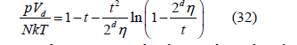
Although the virial expansion provides an almost exact description of a gas of hard spheres, it is not a simple expression well suited to find a simple equation of state for real gases. Therefore, the power law (29) remains interesting. We have searched for a power law that approximates the free-volume function obtained through (27) from the virial coefficients given in [25]. We found that the best exponent is t = 8/3 as shown in Figure 11. For this exponent, the largest difference between the power law and the free-volume function obtained from the virial expansion is 0.011, and the freevolume function (29) and the compressibility factor (32) become

which differ from f (η ) =1−8η +17η ² +.... and pV / (NkT) =1+ 4η +10η ² +... calculated by Van Laar and Boltzmann. This is the price to pay for having a power law that approximates the free-volume function well enough for all coverages. The power law provides an easy expression of the compressibility factor. On the other hand, the power law (29), although approximate, gives a positive answer to the question of whether the virial coefficients are all positive, because the compressibility factor (32) contains a logarithm whose expansion only provides positive terms for any positive exponent t. On the other hand, it must be noted that any virial expansion is not valid beyond the radius of convergence, which is the maximum of 𝜂. Since only a finite number of virial coefficients are known, the radius of convergence cannot be calculated, but an estimate can be found from the quotient of virial coefficients, which are 4, 2.5, 1.8365, 1.5369, 1.4107, 1.3397, 1.2847, 1.2524, 1.2313, 1.2017 and 1.0472 from B2 / B₁ to B₁₂ / B₁₁ according to [25]. The last quotient is not reliable because B₁₂ still has a lot of uncertainty. The filling of a close-packed lattice of spheres is ψ_comp =1 and then , which should be the radius of convergence for the virial series. It implies that

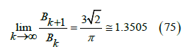
Figure 11:Free-volume function calculated from the virial coefficients by means of (27) (squares) and from the power law (29) (curve) with exponent t = 8 / 3 against the packing fraction.

The singularity and the radius of convergence of the virial series have been discussed in [26]. In our simulations, the free volume becomes zero about ψ _max ≈ 0.57 on average, and η_max ≈ 0.42 . Anyway, close to η_max , the phase transition towards a solid ordered lattice takes place. Monte Carlo and molecular dynamics simulations [20,27] show that freezing occurs at η = 0.49 , melting occurs at η = 0.539 and the maximum random packing fraction appears to be max η_max = 0.64 . The power law with exponent 8/3 predicts η_max =1/ 3 ≅ 0.3333 , where the compressibility factor (74) becomes infinite. For η = 0.42 , the compressibility factor given by the virial expansion is only 7.81.

The compressibility factor can be calculated from the twelve virial coefficients given in [25]. However, a simpler expression can be found for use in the graphs of the compressibility factor. We have found that the exponential function

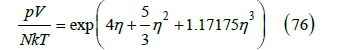
fits the compressibility factor calculated from the virial expansion very well, as shown in Figure 12. The difference between the two values of the compressibility factor for 0 ≤η ≤ 0.74 is less than or equal to 0.6%. The expansion of this exponential gives

Figure 12:Logarithm of the compressibility factor versus the packing fraction. Curve calculated from the virial expansion (26). Squares calculated from the exponential function (77).

that is, B₂ = 4 , B₃ ≅ 9.6667 (exact value 10), B₄ =18.5.51 (exact value 18.3648), and 5 B ≅ 30.0759 (exact value 28.2244). From (76), however, no easy algebraic expression for the free-volume function can be found. On the other hand, this exponential function does not have the expected singularity. Anyway, it provides better values of the compressibility factor than the potential law.

Soft spheres and the lennard-jones potential

Real gases cannot be completely described by a hard-sphere gas. However, some conclusions obtained from this model can be applied to real gases with appropriate adaptation. The first approximation to the behavior of real gases was the van der Waals equation. This equation incorporates two features, an attractive term added to the pressure, and a co-volume of molecules which is subtracted from the gas volume. The van der Waals equation predicted the critical point and the corresponding states: a universal equation of state written with reduced pressure, volume and temperature obtained by dividing by their critical values holds for all real gases. This is a very good approximation for real gases, but the experimental plot differs from that calculated using the van der Waals equation. The hard-sphere gas modifies the van der Waals correction of covolume, since it is clear that the occupied volume is not the sum of the exclusion volumes of hard spheres except at low densities. However, the hard-sphere radius of real gases is not constant and depends on the temperature. In fact, molecules behave like hard spheres only at low temperatures and like elastic spheres at higher temperatures. On the other hand, attractive van der Waals forces are not included in the hard-sphere model, so they must be incorporated in some way. We did it in [12], and we now briefly explain these modifications. The second virial coefficient of the expansion of the pressure in terms of the density

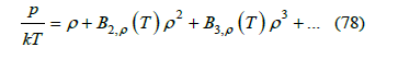
is calculated (in three dimensions) as the integral [28]

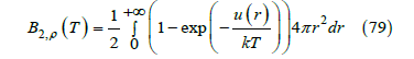
Where u(r) is the potential energy as function of the distance r between the centers of two molecules. Since two centers of hard spheres cannot approach a distance less than 𝜎 = 2R, the potential energy for the hard-sphere gas is

For this hard-sphere potential, the calculated virial coefficient is B _2,ρ = 2πσ³/3 , which corresponds to B₂ = 4 in the virial expansion of the compressibility factor (26) in terms of the packing fraction 𝜂.

In order to go beyond the hard-sphere model, we chose Lennard-Jones potential, which well approximates the power laws of intermolecular interaction at long and short distances

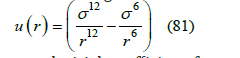
To calculate the second virial coefficient from the Lennard- Jones potential, we split the integral (79) into two intervals, one repulsive ( 0 < r <σ ) and other attractive ( r >σ )

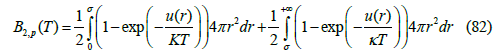
The strategy of separating the repulsive and attractive parts of the intermolecular potential is frequently used in the literature [29]. It allows us to find different analytic approximations.

The expansion of the exponential in the second integral of (82), which is possible because −4ε ≤ u(r) ≤ 0 in the attractive interval and usually ε / kT ≤1 for the gas phase, gave rise to [12, Equation 52] (Appendix)

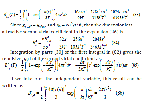
because u(0) = +∞ and u(σ ) = 0. Taking r as the unknown in the Lennard-Jones potential (81), the function r(u) is found as the solution to that equation for r < 𝜎

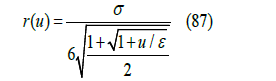
r(u) is the shortest distance to which the centers of two spheres with relative energy u can approach each other, which depends on the energy level as shown in Figure 13. The higher the energy, the smaller the radius of maximum approach. Therefore, with the Lennard-Jones potential, hard spheres become soft spheres like elastic balls, a model which better approximates real gases. The Lennard-Jones potential describes elastic energy as a function of the distance between the centers of two balls during a collision. {r³} can be interpreted as the average of the cubic power of this shortest distance for different energies following the Gibbs distribution [31]

Figure 13:Reduced Lennard-Jones potential as a function of the reduced distance between the centers of two spherical molecules. The horizontal lines indicate a few levels of relative energy. The higher the relative energy, the smaller the minimum distance they can reach (the radius of the exclusion sphere).

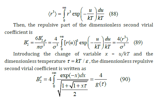
where g(τ ) is a function that tends to unity at zero temperature. Since the integral cannot be integrated analytically, we have sought and found an approximation to g(τ ) with the help of numerical integration

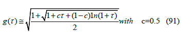
The goodness of this approximation is shown in Figure 14. Although the best fit that minimizes the sum of the squares of the differences is obtained for c = 0.507818922, we choose c = 0.5 for simplicity.

Now, the repulsive second term in the virial expansion of the compressibility factor is

Figure 14:The repulsive part of the second virial coefficient B₂ divided by 4 for the Lennard-Jones potential (81) against kT /ε . Squares calculated from Simpson’s numerical integration of (90) with step Δx = 0.1. Curve calculated with the approximation (91) of g (τ ) .

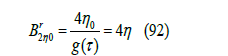
where η₀ =πσ³ / 6 is the packing fraction for an exclusion radius 𝜎 and T = 0. By adding the attractive part (84) and the repulsive part (92), the dimensionless second virial coefficient can be approximated by

Τ = 0 (93)

Table 2 shows the reliability of this analytic approximation to B2, as its difference from the exact values of the numerical integration in [15, Appendix] is 1% or less. Here some errors in the second and third columns of [12, Table 2] have been corrected. The exact analytic expression for B2 for the Lennard-Jones potential has been given as a linear combination of modified Bessel functions [30]. However, the algebraic approximation (93) remains useful, since it is much easier to implement and calculate than the modified Bessel functions.

Table 2:Second virial coefficient.

^a Obtained from numerical integration. Some errors in [12, Table 2] have been corrected here.

The variable 𝜂 in (92) can be interpreted as a packing fraction like 𝜂₀ but corresponding to the dimensionless temperature 𝜏

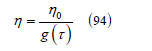
The exclusion radius at a certain temperature T =ετ / k is smaller than the exclusion radius 𝜎 at zero temperature, that is, real gases can be considered as a gas of soft spheres with an average exclusion radius that depends on the temperature. Therefore, Figure 14 also displays how the exclusion volume of a spherical molecule decreases as the temperature increases. If we introduce the variable z = 𝜎³ / r³, the attractive part of the second virial coefficient can be written as the integral

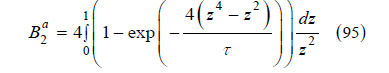
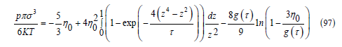
We use the numerical evaluation of this integral instead of the approximation (84) to achieve more precision in determining the critical point. By introducing 𝜂 (94) into (74) and adding the attractive part of the second virial coefficient (95), we obtain how the free-volume function and the compressibility factor depend on temperature

This equation of state satisfies the principle of the corresponding states: after dividing the pressure, temperature and molar volume by their critical values, a single equation of state is obtained for the reduced magnitudes. To find the critical parameters, we write the pressure as function of η₀ = Nπσ³ / (6V )

The critical point is the horizontal inflection point of the graph of pressure versus volume V or versus 𝜂₀, which is inversely proportional to V. By setting the first and second derivatives equal to zero, we find

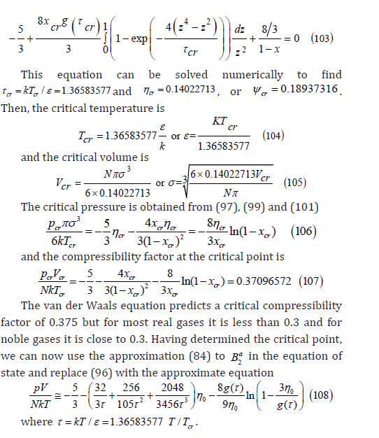
The compressibility factor calculated from (108) is plotted versus the reduced pressure p/ p_cr in Figure 15 for the reduced temperatures / cr T T equal to 1, 1.1, 1.2, 1.3, 1.5, and 2. When these curves are compared with common experimental curves obtained for various real gases [32-37], it is seen that the calculated minima (0.30, 0.47, 0.60, 0.69, 0.82, and 0.97) are higher than the experimental minima (0.22, 0.40, 0.55, 0.65, 0.80 and 0.96) and occur at lower reduced pressures (1.12, 1.82, 2.25, 2.67, 2.97, and 2.50) than the experimental ones (1.2, 2, 2.6, 3.0, 3.5, and 3). On the other hand, the calculated values of the compressibility factor in the zone of linear behavior at high pressures (right of Figure 15) are higher than the experimental values, for example, for natural gas [38, Figure 1]. The intersection pattern of the linear variations is similar, but the calculated curves cross for reduced pressures comprised between 5 and 8 while the experimental curves do so for reduced pressures between 7 and 11 or so. The conclusion of this comparison is that our equation of state (108) underestimates the attractive forces but describes well the variation of the free volume and the effective exclusion radius with temperature. This makes sense because this equation of state incorporates only the attractive part of B2 but omits the attractive parts of other virial coefficients. The repulsive part of all virial coefficients seems to be well described by the effective exclusion radius, whose temperature dependence is already included in the equation of state (108). In [12], we calculated the exclusion volume assuming the Maxwell-Boltzmann distribution for the relative velocities, instead of Equation (89) similar to the Gibbs distribution. Due to incorrect boundary conditions, we also took an exponent 3.2 for the potential law of the free-volume function instead of the correct value 8/3. Despite these two erroneous assumptions that have now been corrected, the conclusions were similar to those found here. The fact that variations in the energy distribution or the power law exponent do not substantially modify the compressibility factor curves is an indication that an additional attractive term is needed. Therefore, further research on the attractive parts of higher virial coefficients will be carried out in the future.

Figure 15:Compressibility factor calculated from Equation (108) as a function of the reduced pressure for the reduced temperatures T / T_cr equal to 1, 1.1, 1.2, 1.3, 1.5 and 2 (curves from bottom to top).

The ionic adsorption isotherm

This section deals with the adsorption of ions in the presence of an electric field across the interface, whose description is more complex than that given by the Langmuir isotherm or the billiard model. In general, an adsorption isotherm for a two-dimensional hard-sphere gas of ions is given by

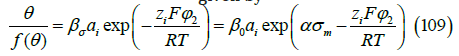
where the Faraday constant is F = 96,485.322.....C/mol [39], and the gas constant³ is R = 8.314462....J.mol⁻¹ K⁻¹ . The adsorption coefficient σ β depends on the metal charge, so β₀ is the adsorption coefficient at zero metal charge. With the modified Frumkin isotherm (5), which includes the same electric factors as on the right-hand side of (109), we reproduced [8] the adsorption of chloride and iodide at constant ionic strength and at varying ionic strength, as well as the capacity curves using the thermodynamic relation

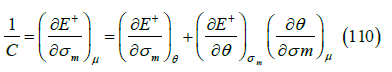
where C is the interfacial electric capacity (in F/m²), E⁺ (in V) is the electrode potential of a cation-reversible electrode (if the adsorption of an anion is measured), and 𝜇 is the chemical potential in the solution. The capacitance is usually measured by applying a small oscillation to the electrode potential. The change in E⁺ means that the coverage also changes by adsorption and desorption at constant chemical potential. This process is slow in comparison with the very fast dielectric response of the adsorption layer, so the capacitance depends on the frequency of the oscillation applied to E⁺. C is the extrapolation of the capacitance at zero frequency. A model of diffusion-limited complex capacitance was given in [40]. The partial derivative

can only be measured at high frequencies where changes in adsorption are limited by diffusion, although this derivative has sometimes been confused with the capacity at zero frequency. As the frequency increases further, a point is reached where the dielectric relaxation cannot keep up with the oscillation of the electric field. The relative permittivity of the adsorption layer is very low, around 6 [10], while that of liquid water is around 78 (at room temperature). Liquid water has two dielectric relaxation processes [41]. At 298.15K, the complex dielectric constant is the sum of two relaxation processes with amplitudes of 72 and 1.75, and relaxation times of 8.38ps and 1.1ps respectively plus an amplitude of 4.57 at infinite frequency (total dielectric constant of 78.32). The main relaxation process is due to the motion of protons in the quantum regime along chains of water molecules following Fermi-Dirac statistics [42]. Because adsorbed water chains are expected to be parallel to the surface, the motion of protons cannot respond to variations in the electric field applied perpendicular to the interface. Therefore, only the second dielectric relaxation mechanism of liquid water can account for the polarization of water molecules in the adsorption layer. This gives a dielectric permittivity of 1.75+4.57=6.32, close to the observed value 6.73 (see below). In our opinion, the reorganization of the external protons, those not involved in hydrogen bonds of the water chains, together with the polarizability of the electron clouds explain the low dielectric constant of the interface.

³ The constants F and R can be replaced by the elementary charge e and the Boltzmann constant k, whose values are exact [39], although this is not useful because experimental errors in adsorption studies are much higher than rounding errors in F and R.

The form of the adsorption isotherm (109) is not capricious. De Levie [43] introduced the Boltzmann factor z_i Fϕ₂ / (RT) to correct the Frumkin isotherm for ionic adsorption. This factor can be understood in two equivalent ways. The electric potential is a continuous function of the distance to the metal surface. Thus, the electric potential at the plane where the centers of the adsorbed ions are located, the inner Helmholtz plane (IHP), is the addition of a potential drop across the interphase (the adsorbed phase) and the electric potential at the boundary of the diffuse layer, the outer Helmholtz plane (OHP). The electric potential at the OHP, also called the diffuse layer potential, is just ϕ₂ taking the electric potential at the bulk solution as zero. Therefore, the ionic electrochemical potential in the adsorption layer is the sum of the interfacial chemical potential due to coverage, the electric potential drop between the IHP and the OHP times , and z_i Fϕ₂ . Equilibrium between the adsorption layer and the bulk solution implies that the interfacial electrochemical potential equals the chemical potential in the bulk solution leading to the ionic adsorption isotherm with the Boltzmann factor. The other way to understand the Boltzmann factor is to assume that equilibrium implies equality of chemical potentials in the adsorption layer and at the OHP. Of course, the ionic concentration at the OHP differs from the ionic concentration at the bulk solution owing to the polarization of the diffuse layer. The constancy of the electrochemical potential across the diffuse layer yields equality

and thus, the Boltzmann factor enters the adsorption isotherm.

The term ασ_m accounts for the variation of ln β_σ with the metal charge σ_m , which is approximately linear for many ions. This term and the Boltzmann factor are thermodynamically linked to Grahame’s electric model of the double layer. Let us give more details. Dutkiewicz et al. [44] studied the adsorption of iodide on mercury from solutions of x M KI + (1-x) M KF, where x is the iodide molar fraction. Under the assumption that the surface excesses of iodide in the diffuse layer and fluoride are proportional to their concentrations (it is assumed that fluoride is not specifically adsorbed)

The electrocapillary equation at constant ionic strength directly gives the surface excess of specifically adsorbed iodide. This assumption is more general than the Gouy-Chapman theory and is also satisfied by other alternative theories such as the compatible theory [45]. On the other hand, since the concentration of the cation K+ and the ionic strength are constant, the variation of the potential of a cation-reversible electrode is equal to the variation of the potential of a reference electrode such as the normal calomel electrode (NCE⁴) with which the experimental measurements were carried out, that is, dE⁺ = dE_NCE . Therefore, for adsorption at constant ionic strength such as Dutkiewicz’s system, the electrocapillary equation is

where is the specifically adsorbed surface excess of the ion i, E is the electrode potential with respect to a reference electrode such as NCE, SCE or NHE (normal hydrogen electrode), and due to the constancy of the activity coefficients at constant ionic strength⁵. Parsons defined the Legendre transform ξ =γ +σ_m E of the surface tension in order to replace E by σ_m as the independent electric variable. Similarly, we defined the function⁶ [8] in order to replace the chemical potential by the surface excess as the independent chemical variable. Its differential is

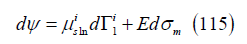
The integration of the ionic adsorption isotherm (109) with respect to the surface excess at constant metal charge taking into account that the diffuse layer potential is only a function of the diffuse layer charge7, that is, 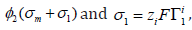, gives

⁴ The normal calomel electrode (NCE) is a reference electrode with a solution of 1N KCl in equilibrium with Hg2Cl2 (calomel). The saturated calomel electrode (SCE) has a saturated KCl solution. The potentials with respect to both electrodes differ by 27mV.
⁵ At constant ionic strength, the activity coefficients are approximately constant and their variation with the ratio of iodide to fluoride can be neglected.
⁶ Here 𝛹 is a Legendre transform of the surface tension which should not be confused with the filling.
⁷ The charge of the diffuse layer is opposite to the addition of the metal charge and the adsorption charge, 𝜎_d = 𝜎₁+𝜎_m, due to the condition of electroneutrality of the interface.

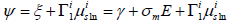
where h(σ_m ) is an arbitrary function of the metal charge. The partial derivative of 𝛹 with respect to the metal charge is the electrode potential

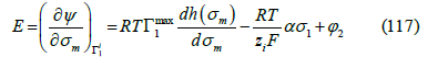
Thus, the electrode potential is the diffuse layer potential plus an electric potential drop across the inner part of the interface that includes a potential drop due to adsorption and another due to metal polarization (plus a constant), as we expected from the fact that the electric potential is a continuous function of the coordinate perpendicular to the interface. Therefore, the Boltzmann factor in the adsorption isotherm is thermodynamically linked to the electric potential drop across the diffuse layer. To see that the term ασ_m in the adsorption isotherm is also thermodynamically linked to the potential drop across the adsorption layer, let us recall that Grahame [46] modeled the interface as a condenser of three plates (Figure 16): the metal surface (0), the IHP (1), where the centers of the adsorption charges are located, and the OHP (2), which is the boundary of the diffuse layer. Applying the Gauss theorem to this capacitor, we find [9]

Figure 16:Grahame’s model of the electric double layer like a condenser of three plates: the metal surface (0), the IHP (1), and the OHP (2), which is the boundary of the diffuse layer.

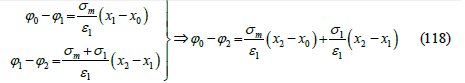
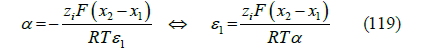
With x₀ < x₁ < x₂ , where 𝜀1 is the absolute permittivity of the inner layer between the metal surface and the OHP. The identification of the two second terms in (117) and (118) gives

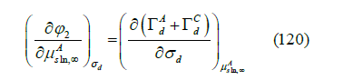
The diffuse layer is the zone of polarization of the solution. The diffuse layer potential 𝜙₂ is the difference of electric potential between the OHP and the bulk solution. It is usually calculated using the Gouy-Chapman theory. However, we proved [45] that any theory of the diffuse layer must satisfy the thermodynamic compatibility equation. For a symmetric z : z electrolyte, under the approximation that the activities of the anion and cation are the same in the bulk solution, the compatibility equation can be obtained [47] from the Schwarz theorem of equality of mixed partial derivatives

of the addition of the Parson’s functions ξ₊ + ξ₋ for an ideal nonadsorbed electrolyte (for more details see [40,45]). are the surface excesses of the anion and cation in the diffuse layer, and σ_d= zF(Γ_C− Γ_A) is the diffuse layer charge. The Gouy-Chapman theory, which is based on the constancy of ionic electrochemical potentials given by 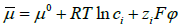across the diffuse layer, only satisfies the compatibility equation (120) for dilute solutions, but not for concentrated solutions, where chemical potentials are the logarithms of activities that differ from concentrations. Our compatible theory of the diffuse layer [45] based on the constancy of the electrochemical potentials

and tending to the Gouy-Chapman theory in dilute solutions predicts, for a symmetric z : z electrolyte, the diffuse layer potential

where σ_d = −σ_m −σ₁ is the diffuse layer charge, ε_sln is the absolute permittivity of the solution, and is the mean ionic activity in the electrolyte solution at infinite distance from the electrode, which replaces the total salt concentration of the Gouy- Chapman theory. In the deduction, it is assumed that the anion and cation have the same ionic activity in the bulk solution, but their activity coefficients differ in the diffuse layer. The theory can be extended to asymmetric electrolytes, which we did in [45]. Damaskin and Grafov [48] verified the goodness of the compatible theory for aqueous solutions of Na₂ SO₄ and La₂(SO₄)₃ on mercury.

Just as the diffuse layer is the polarization zone of the solution, the metal electrode also has a polarization zone near the metal surface. Metal polarization can be well described by the Rice model [49]. In this model, the crystal lattice of metal ions is approximately described by a continuum of positive charge (jellium), and the Fermi statistics is applied to the electrons in the conduction band. The electrochemical potential of the electrons in the metal is assumed to be constant and equal to the sum of the Fermi energy ∈_F plus the electric potential inside the metal m ϕ ∞ times the electron charge e

where c_e( x) and are the conduction electron concentrations at a finite distance x and an infinite distance from the metal surface. This equation is an approximation at the limit T →0 , since at room temperature kT <<∈_F . This condition together with the Poisson equation [9] leads to

where ϕ₀ is the electric potential at the metal surface, is the electric potential in the metal at infinite distance from the electrode surface, 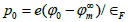is the reduced electric potential at the metal surface, 𝜀₀ is the vacuum permittivity, and

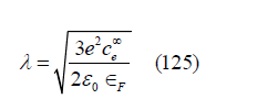
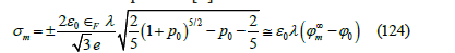
is the inverse of the thickness of the polarization layer. When p₀ < 0 , then . The linear approximation in (124) is justified by the fact that the Fermi energy of the electrode metals usually ranges between 5 and 8eV, while the usual polarization potential of electrochemical experiments ranges up to ±1V from the potential of zero charge. Under this approximation, the capacity is constant 0 C =ε λ , and the electric potential drop has an exponential profile in the metal

The exact capacity is obtained as the derivative of (124) with respect to the electric potential

This capacity is independent of temperature and decreases slowly from negative to positive metal charges. This behavior has been observed at the mercury/aqueous solution interface. Grahame [50] showed that the capacity curves of the mercury electrode at negative metal charges are independent of temperature and, in fact, do not depend on the nature of the anion or the cation if it is small enough like Na⁺ or K⁺. For solutions of NaF on mercury, the inner layer capacity curves, whose inverse is the subtraction of the inverse of the diffuse layer capacity from the inverse of the total capacity, are coincident from very negative metal charges up to -0.12C.m^-2 where they begin to change with temperature (which varies between 0º and 85 ºC) increasingly towards more positive charges. The Rice model predicts, at −0.20, −0.16, and −0.12C.m^-2 for two conduction electrons per mercury atom measured from the Hall effect [51], capacities of 0.1636, 0.1627, and 0.1618F.m^-2, while the observed inner layer capacities are 0.198, 0.18, and 0.16F.m^-2 respectively. For other metals, the values of the capacity in the absence of adsorption are similar to the values calculated from the Rice model, although the fit is not exact. If we combine the compatible theory, the Grahame model and the linear approximation of the Rice model, the electrode potential should be

The constant K depends on the reference electrode. It should be noted that this electrode potential assumes the approximation of linear dielectric response of the solvent (usually water) in the diffuse layer and in the inner layer between the OHP and the metal surface. As explained above, the electrode potential (128) is thermodynamically consistent with the ionic adsorption isotherm (109).

Let us see how we tested [10] the billiard isotherm with halide adsorption data. Taking logarithms in (109), we have

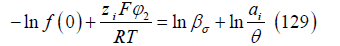
That is, the plot of at constant metal charge should be linear with unity slope. The adsorption of chloride on mercury from aqueous x KCl +(1-x) KF [52] plotted using the Langmuir isotherm and the Gouy-Chapman theory give slopes less than or equal to 0.82 [8, Table 2]. The billiard isotherm together with the compatible theory yields the slopes 0.8500, 1.0883, 1.1032, and 1.0744 at the metal charges of 0, 0.04, 0.08, and 0.12C.m^-2 respectively. The linear regression of the four values of ln β_σ so obtained against the metal charge m σ yields α =118.20m2C⁻¹ with a very good correlation coefficient. Under the assumption that the distance between the IHP and the OHP is equal to the chloride ionic radius, , one obtains an absolute permittivity between both planes of , which is a relative permittivity of ε_r = ε₁ / ε₀ =6.73 much lower than 78.5 for water at 25 ºC as previously discussed. The plots of iodide adsorption on mercury from aqueous x KI+(1-x) KF [44] by using the Langmuir isotherm and Gouy-Chapmen theory give slopes less than 0.34, equivalent to a repulsive interaction parameter in a Frumkin isotherm such as the one we used in [8]. The billiard isotherm and compatible theory increase the slopes to 0.4205, 0.4356 and 0.4250 at the metal charges of −0.06, −0.08 and −0.10 C.m-2, which are far from unity. Our first interpretation of this result was that dielectric saturation of the medium between the IHP and the OHP begins to occur because the diffuse layer charges for iodide adsorption are higher than for chloride adsorption. However, a quantitative explanation has not yet been given, and it can still be considered an open question. This shows that checking the billiard isotherm is quite complex for ions due to the interfacial electric field. Even for neutral compounds, the electric field cannot be ignored. The adsorbed neutral compounds behave as a dielectric material placed between the metal surface and the OHP, but with the particularity that the minimum electric energy and the maximum adsorption from aqueous solutions do not occur at zero metal charge as expected but at negative metal charges as shown in [9, Table 1].

Conclusion

The adsorption isotherm derived from the billiard model describes a two-dimensional gas of hard spheres whose molecules are free to translate. This model is complementary to the Langmuir isotherm, which describes localized adsorption of a denser phase. Both isotherms reproduce the observed phase transition between a more dilute phase and a more concentrated ordered phase of anions. In the billiard model, each spherical molecule occupies four times its own area, and the free-area function decreases with increasing coverage much faster than predicted by the Langmuir isotherm, and not linearly. The free-area function has been obtained from simulation and has been approximated by a coverage polynomial and a power law. The generalization of the billiard model to three dimensions is the hard-sphere gas. In three dimensions, each sphere occupies eight times its own volume, and the free-volume function decreases as the packing fraction increases faster than predicted by the van der Waals equation, and not linearly. Using statistical thermodynamics, the equation of state of a hard-sphere gas for a given free-volume function has been obtained from the translational partition function of a system of particles whose available volume progressively decreases as more particles are added to the system. The free volume can then be expressed as a function of the virial coefficients in the expansion of pressure in terms of density. The free-volume function obtained from the virial coefficients agrees perfectly with that obtained from our simulations. With the help of a power law that approximates the free-volume function, an equation of state of a hard-sphere gas has been derived. The molecules of real gases are not really hard but are somewhat elastic and attract each other. The Lennard-Jones potential has been taken as the model of intermolecular interaction. It shows how the radius of the exclusion sphere decreases with temperature (hard spheres correspond to zero temperature) and also describes attraction between molecules at longer distances. The equation of state of the hard-sphere gas obtained from the power law with a temperaturedependent exclusion radius and the attractive part of the second virial coefficient qualitatively describes the observed universal curves of the compressibility factor versus the reduced pressure, although the agreement is not yet quantitative. Finally, the ionic adsorption isotherm that takes into account the drop in the electric potential across the interface is reviewed, as well as its application to the study of halide adsorption, which led us to the billiard model.

Appendix

Polynomial approximation to the attractive part of the second virial coefficient for the lennard-jones potential

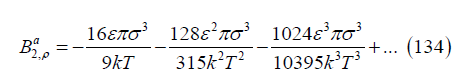
To calculate the attractive part of the second virial coefficient for the Lennard-Jones potential, integration is performed for the interval r > 𝜎

Close to the critical point, ε / (kT) ≅ 0.73, ε ² / (k² T ² ) ≅ 0.54 and ε ³ / (k³ T³ ) ≅ 0.39 so that the coefficients of 𝜎3 are 0.6508, 0.1089 and 0.0193, which shows that the series has good convergence. For temperatures above the critical temperature, the convergence is better. Therefore, the attractive part of the second virial coefficient is

This expansion can be continued if desired by calculating more terms.

References

1. Mende D, Simon G (2005) Physik. Fachbuchverlag Leipzig im Carl Hansen Verlag, München, Germany, p. 157.
2. Eggert J, Hock L (1943) Tratado de Química Fí (2^nd edn), Labor, Barcelona, Spain, p. 325.
3. Glasstone S (1979) Tratado de Química Fí (7^th edn), Aguilar, Madrid, Spain, p. 265.
4. Damaskin BB, Petrii OA, Batrakov VV (1971) Adsorption of organic compounds on electrodes. Plenum Press, New York, USA, p. 86.
5. Langmuir I (1918) The adsorption of gases on plane surfaces of glass, mica and platinum. J Am Chem Soc 40 (9): 1361-1403.
6. Frumkin AN (1925) Die Kapillarkurve der höheren Fetsäuren und die Zustandsgleichung der Oberflä Z Phys Chem 116(1): 466-484.
7. Lust K, Väärtnõu M, Lust E (2000) Adsorption of halide anions on bismuth single crystal plane electrodes. Electrochim Acta 45(21): 3543-3554.
8. Sanz F, González R (1989) Theoretical considerations on the adsorption isotherm for ionic systems at electrode interphases. Electrochim Acta 34(12): 1883-1887.
9. González R (2006) Applications of the thermodynamic method to the study of electrochemical interfaces. Curr Top Electrochem 11: 93-116.
10. González R (2025) Adsorption isotherm deduced from the billiard model. Electrochim Acta 524: 145917, 1-10.
11. Magnussen OM (2002) Ordered anion adlayers on metal electrode surfaces. Chem Rev 102(3): 679-725.
12. González R (2025) Equations of state of a two-dimensional and three-dimensional gas of rigid spheres. In: Perspectives and innovation in chemical research. Atena Editora, Brazil, pp. 53-76.
13. Finch C, Clarke Th, Hickman JJ (2013) A continuum hard-sphere model of protein adsorption. J Comput Phys 244: 212-222.
14. Adamczyk Z, Weroński P, Musiał E (2002) Irreversible adsorption of hard spheres at random site (heterogeneous) surfaces. J Chem Phys 116(11): 4665-4672.
15. Díaz Peña M (1979) Statistical Thermodynamics. Alhambra, Madrid, Spain.
16. Speedy RJ (1977) Accurate theory of the hard sphere fluid. J Chem Soc Far Trans 2: Molecular and Chemical Physics 73(5): 714-721.
17. Boltzmann L (1898) On the characteristic equation of vd Waals. Koninklijke Nederlandsche Akademie van Wetenschappen Proceedings 1, pp. 398-404.
18. Boltzmann L (1995) Lectures on Gas Theory. Dover, Mineola, USA, p. 352.
19. Clisby N, McCoy BM (2006) Ninth and tenth order virial coefficients for hard spheres in D dimensions. J Statis Phys 122(1): 15-57.
20. Tian J, Jiang H, Gui Y, Mulero A (2009) Equation of state for hard-sphere fluids offering accurate virial coefficients. Phys Chem Chem Phys 11(47): 11213-11218.
21. Randles JEB, Behr B (1972) Adsorption at fluid interfaces: I. Surface tension at the interface between a binary liquid mixture and its vapour. J Electroanal Chem 35(1): 389-404.
22. Tonks L (1936) The complete equation of state of one, two and three-dimensional gases of hard elastic spheres. Phys Rev 50(10): 955.
23. Janse van Rensburg EJ (1993) Virial coefficients for hard disks and hard spheres. J Phys A: Mathematical and General 26(19): 4805-4818.
24. Hemmer PC (1965) Virial coefficients for the hard-core gas in two dimensions. J Chem Phys 42(3): 1116.
25. Tian J, Jiang H, Mulero A (2019) Equations of the state of hard sphere fluids based on recent accurate virial coefficients B₅-B₁₂. Phys Chem Chem Phys 21(24): 13070-13077.
26. Maestre MA, Santos A, Robles M, López de Haro M (2011) On the relation between virial coefficients and the close packing of hard disks and hard spheres. J Chem Phys 134(8): 084502.
27. Pieprzyk S, Bannerman MN, Branka AC, Chudak M, Heyes DM (2019) Thermodynamic and dynamical properties of the hard sphere system revisited by molecular dynamics simulation. Phys Chem Chem Phys 21(13): 6886-6899.
28. Hill TL (1986) An Introduction to Statistical Thermodynamics. Dover, New York, USA, p. 267.
29. Mulero A, Galán CA, Cachadiña I, Cuadros F (2008) Application of hard-sphere and hard-disk equations of state to the weeks-chandler-andersen reference system. In: A. Mulero (Ed.), Theory and Simulation of Hard-Sphere Fluids and Related Systems. Lecture Notes in Physics 753, Springer, Berlin, Germany, p.111.
30. Vargas P, Muñoz E, Rodríguez L (2001) Second virial coefficient for the Lennard-Jones potential. Physica A 290(1-2): 92-100.
31. Vasilyev AM (1994) An Introduction to Statistical Physics. URSS, Moscow, Russia, p. 128.
32. https://engineering.wayne.edu/mechanical/pdfs/thermodynamic-_tables-updated.pdf
33. Kadem L (2025) II.8 Equations of state.
34. Levine IN (2002) Physical Chemistry. (5^th edn), McGraw-Hill, New York, USA, p. 342.
35. Turns SR (2006) Thermal-Fluid Sciences. An Integrated Approach. Cambridge Univ. Press, Cambridge, UK, p. 100.
36. Kontogeorgis GM, Folas GK (2010) Thermodynamic Models for Industrial Applications. From Classical and Advanced Mixing Rules to Association Theories. Wiley, Noida, India, p. 45.
37. Kondepudi D (2008) Introduction to Modern Thermodynamics. Wiley, Chippenham, UK, p. 26.
38. Heidaryan E, Moghadasi J, Rahimi M (2010) New correlations to predict natural gas viscosity and compressibility factor. J Petrol Sci Eng 73(1-2): 67-72.
39. (2026) National Institute of Standards and Technology, The NIST Reference on Constants, Units and Uncertainty.
40. Grafov BM, Elkin VV (1990) Theory of impedance spectroscopy at ideally polarizable electrodes. Soviet Electrochem 26(8): 909-914.
41. Buchner R, Barthel J, Stauber J (1999) The dielectric relaxation of water between 0ºC and 35ºC. Chem Phys Lett 306(1-2): 57-63.
42. González R (2009) Theoretical considerations on the electroreduction of the hydrogen ion at metal electrodes. Curr Top Electrochem 14: 31-65.
43. De Levie R (1971) Anion bridging and anion electrocatalysis on mercury. J Electrochem Soc 118(8): 185C-192C.
44. Dutkiewicz E, Parsons R (1966) The adsorption of iodide ion from aqueous KI+KF of constant ionic strength. J Electroanal Chem 11(2): 100-110.
45. González R, Sanz F (1997) A thermodynamic test of the diffuse layer theory and its implications on electrode kinetics. Electroanalysis 9(2): 169-175.
46. Grahame DC (1958) Discreteness-of-charge-effects in the inner region of the electric double layer. Z Elektrochem. Berichte der Bunsengesellschaft für physikalische Chemie 62(3): 265-274.
47. Grafov BM, Damaskin BB (1994) Consistency of theoretical models of the electric double layer with the gibbs adsorption equation. Russ J Electrochem 30(12): 1289-1293.
48. Damaskin BB, Grafov BM (1998) Comparing the Gonzalez-Sanz Theory of the Diffuse Layer with the Experimental Data on the Mercury Electrode Capacitance in Aqueous Solutions of Na₂SO₄ and La₂(SO₄)₃. Russ J Electrochem 34(10): 967-971.
49. Rice OK (1928) Application of the fermi statistics to the distribution of electrons under fields in metals and the theory of electrocapillarity. Phys Rev 31(6): 1051.
50. Grahame DC (1957) Capacity of the double layer between mercury and aqueous sodium fluoride. II. Effect of Temperature and Concentration. J Am Chem Soc 79(9): 2093-2098.
51. Cusack N, Kendall P (1961) The hall coefficient of liquid mercury. Philos Mag 6(63): 419-427.
52. Payne R (1968) Specific adsorption of chloride ions at the mercury/aqueous solution interface. Trans Faraday Soc 64: 1638-1655.