
- About Us
- Information
-

The Author ensures that the research has been conducted responsibly and ethically with adherence to all relevant regulations. read more..
- For Authors
- For Reviewer
- Manuscript Guidelines
- Membership
- Publication Ethics
-
- Journals
- Reprints
- e-Books
- Videos
- Policies
- Contact Us
 COVID-19
- Submissions


Full Text
COJ Biomedical Science & Research
Analysis and Control of an Asthma Transmission Model
Lakshmi N Sridhar*
Chemical Engineering Department, University of Puerto Rico, USA
*Corresponding author:Lakshmi N Sridhar, Chemical Engineering Department, University of Puerto Rico, USA
Submission: November 22, 2025; Published: December 19, 2025

Volume2 Issue4December 19, 2025
Abstract
In this study, bifurcation analysis and multi-objective nonlinear model predictive control are performed on an asthma transmission model. Bifurcation analysis is a powerful mathematical tool used to deal with the nonlinear dynamics of any process. Several factors must be considered, and multiple objectives must be met simultaneously. The MATLAB program MATCONT was used to perform the bifurcation analysis. The MNLMPC calculations were performed using the optimization language PYOMO in conjunction with the state-of-the-art global optimization solvers IPOPT and BARON. The bifurcation analysis revealed the existence of branch points. The MNLMPC converged to the Utopia solution. The branch points (which cause multiple steady-state solutions from a singular point) are very beneficial because they enable the Multi objective nonlinear model predictive control calculations to converge to the Utopia point (the best possible solution) in the model.
Keywords:Bifurcation; Optimization; Control; Asthma; Pollution
Background
Ghosh [1], developed a mathematical model concerning industrial pollution and Asthma. D’amato et al. [2], discussed the environmental risk factors (outdoor air pollution and climatic changes) and the increasing trend of respiratory allergy. Martinez FD [3], researched the relationship between genes, environments, development, and asthma. Gauderman et al. [4] studied the effect of traffic on lung development. Ionescu et al. [5,6], developed parametric models characterizing respiratory input impedance and investigated the relationship between fractional-order model parameters and lung pathology in chronic obstructive pulmonary disease. Epton et al. [7] studied the effect of ambient air pollution on the respiratory health of school children. Ram et al. [8] developed a nonlinear mathematical model for Asthma. Strickland et al. [9] studied the short-term associations between ambient air pollutants and pediatric asthma emergency department visits. Ionescu et al. [10,11] performed theoretical work using fractional order models of asthma and respiration. Tawhai et al. [12], developed multi-scale lung models. Annesi-Maesano et al. [13] studied indoor air quality and sources in schools and related health effects. Ionescu et al. [14], developed a respiratory impedance model with a lumped fractional order diffusion compartment. Kim et al. [15] investigated the regulation of Th1/Th2 cells in asthma development. Lim et al. [16], studied the short-term effect of fine particulate matter on children’s hospital admissions and emergency department visits for asthma. Faria et al. [17], studied forced oscillation, integer and fractional-order modelling in asthma. Alejo et al. [18] modelled the association between the seasonal asthma prevalence and upper respiratory infections. Cohen et al. [19] studied the trends of the global burden of disease attributable to ambient air pollution. Ionescu et al. [20] investigated the role of fractional calculus in modeling biological phenomena. Landrigan et al. [21] studied the effect of pollution on children’s health. Whittle et al. [22] studied the molecular characterisation of human dust-mite-associated allergic asthma. Shah et al. [23] developed a mathematical model for Asthma due to Air Pollution. In this work, bifurcation analysis and multiobjective nonlinear model predictive control are performed on a dynamic model describing asthma due to air pollution [23]. The paper is organized as follows. First, the model equations are presented, followed by a discussion of the numerical techniques involving bifurcation analysis and Multiobjective Nonlinear Model Predictive Control (MNLMPC). The results and discussion are then presented, followed by the conclusions.
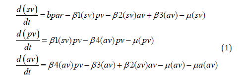
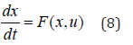
Model equations
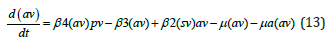
In this model, individuals experiencing an asthma exacerbation are av, individuals affected by indoor smoke are sv, and individuals affected by air pollution are pv. Indoor smoke increases the intensity of pollution in the air at a rate of β1 Asthma-infected individuals infect their surrounding environment at a rate of β3 while the rate at which asthma exacerbation is caused by indoor smoke and outdoor air pollution is β2 and β4 . μa and μ represent the death rate because of asthma exacerbation and a natural degradation rate for all three variables.
The base parameter values are

The variables and parameters can be summarized as
a) individuals experiencing an asthma exacerbation av
b) individuals affected by indoor smoke sv
c) individuals affected by air pollution pv
d) Indoor smoke increases the intensity of pollution in the air at
a rate β1
e) Asthma-infected individuals infect their surrounding
environment at a rate β3
f) rate at which asthma exacerbation is caused by indoor smoke
β2
g) rate at which asthma exacerbation is caused by outdoor air
pollution β4
h) represent the death rate because of asthma exacerbation μa
i) natural degradation rate for all three variables μ
Bifurcation analysis
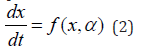
The MATLAB software MATCONT is used to perform the bifurcation calculations. Bifurcation analysis deals with multiple steady-states and limit cycles. Multiple steady states occur because of the existence of branch and limit points. Hopf bifurcation points cause limit cycles. A commonly used MATLAB program that locates limit points, branch points, and Hopf bifurcation points is MATCONT [24,25]. This program detects Limit Points (LP), Branch Points (BP) and Hopf bifurcation points(H) for an ODE system
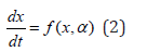
x∈Rn Let the bifurcation parameter be α . Since the gradient is orthogonal to the tangent vector,
The tangent plane at any point w=[w1,w2,w3,w4,....wn+1 ] must satisfy

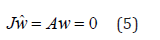
Where ∂f / ∂x is the Jacobian matrix. For both limit and branch points, the Jacobian matrix J = [∂f / ∂x]must be singular.
For a limit point, there is only one tangent at the point of singularity. At this singular point, there is a single non-zero vector, y, where Jy=0. This vector is of dimension n. Since there is only one tangent the vector y=[y1,y2,y3,y4,....yn] must align with ˆw=[w1,w2,w3,w4,....wn]. Since
the n+1th component of the tangent vector wn+1= 0 at a Limit Point (LP).
For a branch point, there must exist two tangents at the singularity. Let the two tangents be z and w. This implies that

Consider a vector v that is orthogonal to one of the tangents
(say w). v can be expressed as a linear combination of z and w (
v =α z +β w). Since Az = Aw = 0 ; Av = 0 and since w and v are
orthogonal, wTv = 0 . Hence  which implies that B is singular.
Hence, for a Branch Point (BP) the matrix  must be singular.
At a Hopf bifurcation point,
 @ indicates the bialternate product while is the n-square
identity matrix. Hopf bifurcations cause limit
cycles and should be eliminated because limit cycles make
optimization and control tasks very difficult.
@ indicates the bialternate product while is the n-square
identity matrix. Hopf bifurcations cause limit
cycles and should be eliminated because limit cycles make
optimization and control tasks very difficult.
More details can be found in Kuznetsov [26,27] & Govaerts [28].
Multiobjective Nonlinear Model Predictive Control (MNLMPC)
The rigorous Multiobjective Nonlinear Model Predictive Control (MNLMPC) method developed by Flores Tlacuahuaz et al. [29] was used.
Consider a problem where the variables 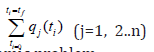 have to be optimized simultaneously for a dynamic problem
tf being the final time value and n the total number of objective
variables and u the control parameter. The single objective optimal
control problem is solved individually optimizing each of the
variables  The optimization of
  will lead to the values q*j. Then, the Multiobjective Optimal Control (MOOC) problem that
will be solved is
will lead to the values q*j. Then, the Multiobjective Optimal Control (MOOC) problem that
will be solved is
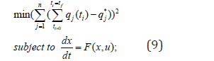
This will provide the values of u at various times. The first
obtained control value of u is implemented and the rest are
discarded. This procedure is repeated until the implemented and
the first obtained control values are the same or if the Utopia point
where  is obtained.
Pyomo Hart et al. [30] is used for these calculations. Here, the differential equations are converted to a Nonlinear Program (NLP) using the orthogonal collocation method The NLP is solved using IPOPT Wächter And Biegler [31] and confirmed as a global solution with BARON Tawarmalani M et al. [32].
The steps of the algorithm are as follows
a) Optimize  and obtain q*j.
b) Minimize 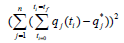 and get the control values at
various times.
and get the control values at
various times.
c) Implement the first obtained control values
d) Repeat steps 1 to 3 until there is an insignificant difference
between the implemented and the first obtained value of the
control variables or if the Utopia point is achieved. The Utopia point
is when 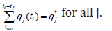 for all j.
Sridhar [33] demonstrated that when the bifurcation analysis
revealed the presence of limit and branch points, the MNLMPC
calculations to converge to the Utopia solution. For this, the
singularity condition, caused by the presence of the limit or branch
points was imposed on the co-state equation Upreti [34]. If the
minimization of 1 q lead to the value q*1 and the minimization of q2
lead to the value q*2 The MNLPMC calculations will minimize the
function 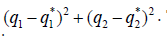 . The multiobjective optimal control
problem is
. The multiobjective optimal control
problem is
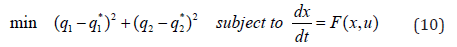
Differentiating the objective function results in
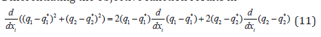
The Utopia point requires that both (q1 − q*1) and * (q2 − q*2) are zero. Hence
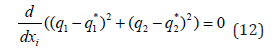
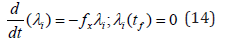
The optimal control co-state equation [34] is
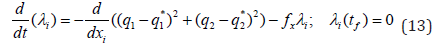
λi is the Lagrangian multiplier. tf is the final time. The first term in this equation is 0, and hence
At a limit or a branch point, for the set of ODE 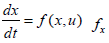 is
singular. Hence there are two different vectors-values for [λi]
where
is
singular. Hence there are two different vectors-values for [λi]
where 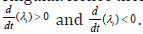 . In between there is a vector [λi]
where
. In between there is a vector [λi]
where  . This coupled with the boundary condition λi(tf) =0 will lead to
[λi] = 0 This makes the problem an unconstrained optimization
problem, and the optimal solution is the Utopia solution.
. This coupled with the boundary condition λi(tf) =0 will lead to
[λi] = 0 This makes the problem an unconstrained optimization
problem, and the optimal solution is the Utopia solution.
Results and Discussion
Theoretical development Theorem
If one of the functions in a dynamic system is separable into two distinct functions, a branch point singularity will occur in the system.
Proof
Consider a system of equations
x∈Rn . Defining the matrix A as
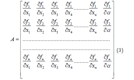
α is the bifurcation parameter. The matrix A can be written in a compact form as
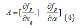
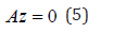
The tangent at any point x; z=[z1,z2,z3,z4,....zn+1 ] must satisfy
The matrix  must be singular at both limit and branch
points. The n+1th component of the tangent vector zn+1 = 0 at a
Limit Point (LP) and for a Branch Point (BP) the matrix
must be singular at both limit and branch
points. The n+1th component of the tangent vector zn+1 = 0 at a
Limit Point (LP) and for a Branch Point (BP) the matrix  must be singular. Any tangent at a point y that is defined by
z=[z1,z2,z3,z4,....zn+1 ] must satisfy
must be singular. Any tangent at a point y that is defined by
z=[z1,z2,z3,z4,....zn+1 ] must satisfy
For a branch point, there must exist two tangents at the singularity. Let the two tangents be z and w. This implies that
Consider a vector v that is orthogonal to one of the tangents (say z). v can be expressed as a linear combination of z and w ( v =α z +β w). Since Az = Aw = 0 ; Av = 0 and since z and v are orthogonal,
zT v = 0 . Hence  which implies that B is singular where
Let any of the functions fi are separable into 2 functions φ1,φ2 as
At steady-state fi(x,α) =0 and this will imply that either φ1 = 0 or φ2 = 0 or both φ1 and φ2 must be 0. This implies that two branches φ1 = 0 and φ2 = 0 will meet at a point where both φ1 and φ2 are 0.
At this point, the matrix B will be singular as a row in this matrix would be

This implies that every element in the row  would be
0, and hence the matrix B would be singular. The singularity in B
implies that there exists a branch point.
would be
0, and hence the matrix B would be singular. The singularity in B
implies that there exists a branch point.
Numerical results
Bifurcation results: When β1 is the bifurcation parameter a branch point occurs at (sv,pv,av, β1) values of (0.333333 0, 0, 0.9) (Figure 1a)
Fgure 1a:Bifurcation diagram (β1 is the bifurcation parameter) revealing a branch point at (sv,pv,av,β1) values of (0.333333 0, 0, 0.9).

Here, the two distinct functions can be obtained from the second ODE in the model

The two distinct equations are

With pv=0, β1=0.9, av=0, μ =0.3; sv =0.33333 both distinct equations are satisfied, validating the theorem.
When β 2 is the bifurcation parameter a branch point occurs at (sv,pv,av, β 2 ) values of (0.333333 0 0 2.4) (Figure 1b). Here, the two distinct functions can be obtained from the third ODE in the model
The two distinct equations are
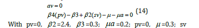
With pv=0, β 2 =2.4, β 3 =0.3; μa =0.2; pv=0, μ =0.3; sv =0.33333, both distinct equations are satisfied, validating the theorem.
Fgure 1b:Bifurcation diagram (β 2 is the bifurcation parameter) revealing a Branch Point (BP) at (sv,pv,av,β 2 ) values of (0.333333 0 0 2.4).

MNLMPC results: For the MNLMPC, β1,β 2, are the control
parameters, and  were minimized individually, and each
led to a value of 0. The overall optimal control problem will involve
the minimization of
were minimized individually, and each
led to a value of 0. The overall optimal control problem will involve
the minimization of 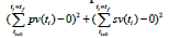 subject to the equations
governing the model. This led to a value of zero (the Utopia point).
The MNLMPC values of the control variables, β1,β 2, were 0.505,
0.00578. The MNLMPC profiles are shown in Figure 2a-2d. The
control profiles of β1,β 2, were exhibited noise (Figure 2c) and this
was remedied using the Savitzky-Golay filter to produce the smooth
profiles β1sg,β 2sg (Figure 2d).
subject to the equations
governing the model. This led to a value of zero (the Utopia point).
The MNLMPC values of the control variables, β1,β 2, were 0.505,
0.00578. The MNLMPC profiles are shown in Figure 2a-2d. The
control profiles of β1,β 2, were exhibited noise (Figure 2c) and this
was remedied using the Savitzky-Golay filter to produce the smooth
profiles β1sg,β 2sg (Figure 2d).
Fgure 2a:MNLMPC pv, sv profiles for the combined
minimization of 

Fgure 2b:MNLMPC av profile for the combined
minimization of 

Fgure 2c:MNLMPC noisy control profiles for β1,β 2 before filtering.

Fgure 2d:MNLMPC β1sg,β 2sg which are filtered noisy profiles of β1,β 2 .

The presence of the branch point causes the MNLMPC calculations to attain the Utopia solution, validating the analysis of Sridhar [33].
Conclusion
It is of utmost importance to understand the dynamics of asthma transmission in order to control it effectively. This study demonstrates the application of integrated bifurcation analysis and MNLMPC to an asthma transmission model, revealing that this integrated approach enables us to understand the nonlinearity and obtain the most control profiles. The proposed link between branch points and optimal control convergence is the main contribution demonstrating a link between applied mathematics, systems biology, and control engineering. The bifurcation analysis revealed the existence of branch points. The branch points (which cause multiple steady-state solutions from a singular point) are very beneficial because they enable the Multiobjective nonlinear model predictive control calculations to converge to the Utopia point (the best possible solution) in the models. A combination of bifurcation analysis and Multiobjective Nonlinear Model Predictive Control (MNLMPC) on an asthma transmission model is the main contribution of this paper.
References
- Ghosh M (2000) Industrial pollution and Asthma: A mathematical model. Journal of Biological Systems 8(04): 347-371.
- D’amato G, Liccardi G, D’Amato M (2000) Environmental risk factors (outdoor air pollution and climatic changes) and increased trend of respiratory allergy. Journal of Investigational Allergology & Clinical Immunology 10(3): 123-128.
- Martinez FD (2007) Genes, environments, development and asthma: A reappraisal. European Respiratory Journal 29(1): 179-184.
- Gauderman WJ, Vora H, McConnell R, Berhane K, Gilliland F, et al. (2007) Effect of exposure to traffic on lung development from 10 to 18 years of age: A cohort study. The Lancet 369(9561): 571-577.
- Ionescu C, De Keyser R (2008) Parametric models for characterizing respiratory input impedance. Journal Of Medical Engineering & Technology 32(4): 315-324.
- Ionescu CM, De Keyser R (2008) Relations between fractional-order model parameters and lung pathology in chronic obstructive pulmonary disease. IEEE Transactions on Biomedical Engineering 56(4): 978-987.
- Epton MJ, Dawson RD, Brooks WM, Kingham S, Aberkane T, et al. (2008) The effect of ambient air pollution on respiratory health of school children: A panel study. Environmental Health 7(1): 16.
- Ram N, Tripathi A (2009) A Nonlinear Mathematical model for Asthma: Effect of Environmental Pollution. Iranian Journal of Optimization 1(1): 24-56.
- Strickland MJ, Darrow LA, Klein M, Flanders WD, Sarnat JA, et al. (2010) Short-term associations between ambient air pollutants and pediatric asthma emergency department visits. American Journal of Respiratory and Critical Care Medicine 182(3): 307-316.
- Ionescu C, Machado JT, De Keyser R (2011) Fractional-order impulse response of the respiratory system. Computers & Mathematics with Applications 62(3): 845-854.
- Ionescu C, Desager K, De Keyser R (2011) Fractional order model parameters for the respiratory input impedance in healthy and in asthmatic children. Computer Methods and Programs in Biomedicine 101(3): 315-323.
- Tawhai MH, Bates JH (2011) Multi-scale lung modeling. Journal of Applied Physiology 110(5): 1466-1472.
- Annesi-Maesano I, Baiz N, Banerjee S, Rudnai P, Rive S, et al. (2013) Indoor air quality and sources in schools and related health effects. Journal of Toxicology and Environmental Health Part B 16(8): 491-550.
- Ionescu CM, Copot D, De Keyser R (2013) Respiratory impedance model with lumped fractional order diffusion compartment. IFAC Proceedings Volumes 46(1): 260-265.
- Kim Y, Lee S, Kim YS, Lawler S, Gho YS, et al. (2013) Regulation of Th1/Th2 cells in asthma development: A mathematical model. Mathematical Biosciences & Engineering 10(4): 1095-1133.
- Lim H, Kwon HJ, Lim JA, Choi JH, Ha M, et al. (2016) Short-term effect of fine particulate matter on children’s hospital admissions and emergency department visits for asthma: A systematic review and meta-analysis. Journal of Preventive Medicine and Public Health 49(4): 205-219.
- Faria AC, Veiga J, Lopes AJ, Melo PL (2016) Forced oscillation, integer and fractional-order modeling in asthma. Computer Methods and Programs in Biomedicine 128: 12-26.
- Alejo AB, Quesada DG (2016) Modeling the association between the seasonal asthma prevalence and upper respiratory infections.
- Cohen AJ, Brauer M, Burnett R, Anderson HR, Frostad J, et al. (2017) Estimates and 25-year trends of the global burden of disease attributable to ambient air pollution: An analysis of data from the Global Burden of Diseases Study 2015. The Lancet 389(10082): 1907-1918.
- Ionescu C, Lopes A, Copot D, Machado JT, Bates JHT (2017) The role of fractional calculus in modeling biological phenomena: A review. Communications in Nonlinear Science and Numerical Simulation 51: 141-159.
- Landrigan PJ, Fuller R, Fisher S, Suk WA, Sly P, et al. (2019) Pollution and children’s health. Science of The Total Environment 650(Pt 2): 2389-2394.
- Whittle E, Leonard MO, Gant TW, Tonge DP (2019) Multi-method molecular characterisation of human dust-mite-associated allergic asthma. Scientific Reports 9(1): 8912-8930.
- Shah NH, Suthar AH, Pandya P (2021) Mathematical modeling for asthma due to air pollution. The Journal of Applied Nonlinear Dynamics 10(2): 219-228.
- Dhooge A, Govearts W, Kuznetsov AY (2003) MATCONT: A Matlab package for numerical bifurcation analysis of ODEs. ACM Transactions on Mathematical Software (TOMS) 29(2): 141-164.
- Dhooge A, Govaerts W, Kuznetsov YA, Mestromand W, Riet AM (2003) Cl_matcont: A continuation toolbox in Matlab. Proceedings of the 2003 ACM Symposium on Applied Computing, Melbourne, Florida, USA, pp. 161-166.
- Kuznetsov YA (1998) Elements of applied bifurcation theory. Springer, Cham, Switzerland.
- Kuznetsov YA (2009) Five lectures on numerical bifurcation analysis. Utrecht University, Netherlands.
- Govaerts WJF (2000) Numerical methods for bifurcations of dynamical equilibria. Society for Industrial and Applied Mathematics (SIAM), USA, p. 362.
- Flores-Tlacuahuac A, Morales P, Toledo MR (2012) Multiobjective nonlinear model predictive control of a class of chemical reactors. I & EC Research 51(17): 5891-5899.
- Hart WE, Laird CD, Watson JP, Woodruff DL, Hackebeil HA (2021) Pyomo-optimization modeling in python (2nd edn), Springer, NY, USA.
- Wächter A, Biegler L (2006) On the implementation of an interior-point filter line-search algorithm for large-scale nonlinear programming. Math Program 106: 25-57.
- Tawarmalani M, Sahinidis NV (2005) A polyhedral branch-and-cut approach to global optimization. Mathematical Programming 103(2): 225-249.
- Sridhar LN (2024) Coupling bifurcation analysis and multiobjective nonlinear model predictive control. Austin Chem Eng 11(1): 1-7.
- Ranjan US (2013) Optimal control for chemical engineers. (1st edn), Taylor and Francis, USA, p. 305.
© 2025 Lakshmi N Sridhar. This is an open access article distributed under the terms of the Creative Commons Attribution License , which permits unrestricted use, distribution, and build upon your work non-commercially.
Editor In Chief


.jpg)


Signup for Newsletter

Quick Links
 Editorial Board Registrations
 Submit your Article
 Refer a Friend
 Advertise With Us
Our Recent Edition

.jpg)


Top Editors


.jpg)


.bmp)
.jpg)
.png)
.jpg)


.jpg)


.png)

.png)


.png)


Financial Support

Sponsors

Latest e-Books

Latest Video

 a Creative Commons Attribution 4.0 International License. Based on a work at www.crimsonpublishers.com.
Best viewed in
a Creative Commons Attribution 4.0 International License. Based on a work at www.crimsonpublishers.com.
Best viewed in