Operator Identification via Recognition of Spectral Branches in Gradient Porous Media

Introduction

The main objective of this paper is to construct a direct model that makes it possible to recover, from experimental data, the spatial-frequency dependence λ=λ(ω) for a gradient porous beam. In the classical wave formulation, one usually analyzes the dependence k=k(ω), where k is the wave number. However, for gradient and defective media, the steady-state response contains both oscillatory and exponential components. Therefore, the more natural object is the full spatial parameter λ, which includes real and imaginary parts.

The model is based on classical works on gradient elasticity [1,2], modern reviews of gradient elasticity and length-scale identification procedures [3], the theory of elastic materials with pores [4], the mathematical theory of defective media [5], and modern nonclassical models of porous beams and plates [6]. The wave interpretation of the obtained solutions is connected with classical results on wave motion in elastic solids [7,8]. Spectral analysis of linear systems and characteristic equations is used in its standard mathematical form [9].

The novelty of the work is as follows:
a) A new interpretation of the inverse problem as a problem of spectral branch recognition is proposed;
b) It is shown that spectral geometry can be regarded as a carrier of information about the system operator;
c) A connection is established between model-parameter identification and recognition of central second-order curves;
d) A representation of dispersion properties through the spatial parameter λ, rather than only through the wave number k, is introduced;
e) It is shown that the measurable characteristics are determined by the roots of the characteristic equation F(λ,ω)=0;
f) For the reversible conservative formulation, a restriction on the form of the branches is formulated: in the variables z=λ² and q=ω² they are central second-order curves without linear terms; the mixed term is absent under additional symmetries of the operator;
g) A scheme for extracting the parameter λ from the spatial structure of the steady-state harmonic response is proposed;
h) The numerical experiment is formulated as recognition of two central second-order branches.

The paper is organized as follows. First, the model is formulated and the kinematic variables of the defective medium are specified. Then the equations of motion and the characteristic equation are derived. After that, the physical meaning of the parameter λ is discussed, a method for extracting it from data is formulated, a scheme for synthesizing the dispersion curve is constructed, and a numerical experiment on recognizing two central branches is performed. In conclusion, a theorem is formulated and proved that relates model-parameter identification to recognition of spectral geometry.

Main results, limitations, and directions for further research.

Problem formulation

A straight beam of length l with a constant cross-section is considered. The coordinate x∈[0,l] is measured along the beam axis, and time is denoted by t. The transverse motion is described by the displacement w(x,t), while the defective structure of the porous medium is described by the internal field φ(x,t).

The dynamics of the system is defined by the Lagrangian

L = T −U, (1)

where T is the kinetic energy and U is the potential energy. Formula (1) fixes a reversible variational formulation without dissipative terms.

The potential energy is written as

where J is the second moment of area of the cross-section, E is the classical bending-stiffness modulus in the adopted normalization, K₁₂ and K₂₂ are local coupling coefficients between porosity and bending deformation, and C₁₁, C₁₂, C₂₂ are gradient coefficients. Energy (2) contains both local and gradient contributions.

The kinetic energy has the form

where ρ is the density, r is the radius of gyration of the crosssection, and ρ₁, ρ₂, ρ₃ are nonclassical inertial densities. Form (3) is consistent with the set of kinematic variables of the model.

Kinematic variables. The deformation state is described by the set of kinematic variables

w(x,t ), ϕ (x,t ), (4)

where w is the transverse displacement and φ is a scalar variable characterizing an incompatible change in the volume of the porous medium. Thus, φ is treated as an independent kinematic variable of the defective medium.

In this sense, the set

{w,w′,w′′,ϕ} (5)

forms the collection of kinematic variables of the defective medium entering the variational formulation of the problem.

Type of support. At the left end x=0, clamping is realized by imposing kinematic constraints on the set (5):

Here W(x) and Phi(x) are the amplitude functions of the harmonic regime, and w₀ is the prescribed displacement amplitude of the clamp.

The condition W’’(0) = 0 in (6) corresponds to the vanishing of the normal derivative of the rotation angle. In gradient bending theory, the moment is not proportional to curvature but is determined by a linear combination of the second and fourth derivatives of displacement and by the contribution of the field φ. Therefore, the condition W’’(0) = 0 has a kinematic rather than a force nature. The support type used here corresponds to a hard-hard clamp, in contrast to a hard-soft variant in which a force condition on the moment is prescribed instead of the second derivative.

At the free end x=l, natural boundary conditions are prescribed; they are obtained from variation of the Lagrangian (1). These conditions correspond to the vanishing of the generalized force factors at the free end.

Equations of motion

We pass to the steady-state harmonic regime and seek the solution in the form

where ω is the excitation frequency, W(x) is the complex amplitude of the transverse displacement, and Phi(x) is the complex amplitude of the internal field.

Substitution of (7) into the Lagrangian system and variation with respect to W and Phi lead to a system of ordinary differential equations in the spatial coordinate. Similar equations arise in problems of wave propagation in elastic media [7,8].

For the displacement W(x) we obtain

and for the internal field Phi(x) we obtain

System (8)--(9) is a higher-order linear system containing derivatives up to the sixth order with respect to displacement and up to the second order with respect to the internal field. This system completely determines the beam dynamics in the harmonic regime and serves as the starting point for constructing the characteristic equation.

Characteristic equation

To construct the spectrum of the system, we seek the solution in the form of exponential functions

where A and B are the amplitudes of the corresponding fields and λ is the spatial spectral parameter.

Substitution of (10) into system (8)--(9) leads to a homogeneous system of algebraic equations for the amplitudes A and B:

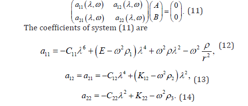
A nontrivial solution of system (11) exists if

Such characteristic equations are a standard tool of spectral analysis for linear systems [9].

Central equation of the model. Equation (15) is treated as the central equation of the model determining the spectrum of the operator.

Introducing the notation

Then characteristic equations (15) is reduced to the form

F (z, q) = 0. (17)

For compact notation, introduce the functions

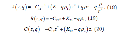
Then the central equation is written as

Analysis of the structure of equation (21) shows that it is quadratic with respect to q:

Hence two dispersion branches follow:

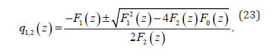
Thus, the spectrum of the system is determined by two branches corresponding to two independent kinematic variables of the defective medium.

Physical interpretation

Characteristic equation (15) defines the spectrum of spatial modes of the system.

In general, the roots of this equation are complex quantities. Therefore, the parameter λ is represented as

λ =α + ik, (24)

where α is the real part characterizing spatial attenuation or growth, and k is the imaginary part determining the wave number.

The corresponding spatial behavior of the solution has the form

which describes decaying or growing wave structures. Thus, each mode of the system is characterized by a pair of parameters (α,k).

Boundary and scale effects. Two types of exponential behavior of the solution should be distinguished, since they have different physical origins.

Boundary effects are already present in classical theory and are related to the geometry of the structure. They appear as exponential attenuation caused by the relation between the beam length and the characteristic lengths arising from boundary conditions.

Scale effects arise in gradient and defective media and are due to the presence of additional length-dimensional parameters entering the model through coefficients at higher derivatives. In this case, characteristic lengths are determined by ratios of moduli of different dimensions.

Introducing the dimensionless parameter

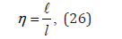
where ℓ is the characteristic length of the scale effect and l is the beam length. For eta≪1, scale effects do not manifest themselves and the behavior of the system is close to classical. For eta∼1, scale effects become significant and determine the structure of the solution.

Thus, the distinction between boundary and scale effects lies in their origin: the former are caused by the geometry of the structure, while the latter are caused by the internal structure of the material and by additional length scales of the gradient model.

Extractable experimental information. If the harmonic response of the beam is measured at a set of spatial points, then the spatial dependence of the complex amplitude can be approximated by a superposition of exponential terms. In the simplest case of a single dominating mode, one obtains

Then the logarithmic derivative makes it possible to recover the parameter λ:

For a complex amplitude, this gives separate estimates for α and k.

Consequently, in contrast to the classical dispersion curve k(ω), the present formulation considers full dependence

λ = λ (ω ), (29)

which contains both wave and attenuating components of the solution. It is precisely this dependence that is the object of the inverse problem in this paper.

Branch analysis and identification

The central equation of the model (21) defines the dispersion structure of the system and determines the set of admissible values of the parameter λ for a given frequency ω.

In an experiment, the spatial structure of oscillations is measured, which makes it possible to recover dependence (29). Passing to variables (16), we obtain that the experimental data are represented by a set of points

which must satisfy the equation

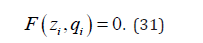
Since the characteristic equation is quadratic with respect to q, the set of solutions is split into two branches

q = q1 (z) , q = q2 (z) . (32)

This means that the experimental points (z_i,q_i) form two families corresponding to different modes of the system.

The problem of identifying the model parameters is formulated as a problem of minimizing the residual

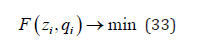
with respect to the model parameters; such a formulation is consistent with the general methodology of inverse problems in dynamics and vibrations [10]. In practice, this requires partitioning the experimental data into two subsets corresponding to different branches, reconstructing the functions q₁(z) and q₂(z), and determining the model parameters from the condition of best agreement with the equation F(z,q)=0.

Method for extracting the parameter λ. The parameter λ is determined from the spatial structure of the steady-state harmonic response. In the steady-state regime, the displacement field is represented as a superposition of modes

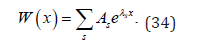
In a region where one mode dominates, the solution is locally approximated by one exponential

Then the parameter λ is determined as the logarithmic derivative

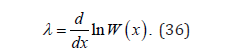
In practice, for sufficiently small Δx, the discrete approximation

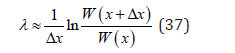
is used. If the complex amplitude is measured, representation (34) is used, where

In the general case, the solution contains several exponential contributions. Then extraction of λ requires localization of a region in which one contribution dominates, or application of procedures for decomposing the response into exponential components. In cantilever problems, it is convenient to use the internal region of the beam for determining the wave numbers k and the vicinity of the clamp for determining the attenuation parameters α, where boundary and scale effects are manifested.

Thus, the identification problem is reduced to recognizing the structure of dispersion branches in the space (z, q) and then recovering the parameters of the operator.

Synthesis of the dispersion curve

The central equation of the model (21) relates the frequency and the spatial parameter and can be used not only for analysis but also for synthesis of dispersion dependences.

The synthesis problem is formulated as follows: for a given set of model parameters, it is necessary to construct dependence (29). For this purpose, at a fixed value of the frequency ω, the characteristic equation

F (λ,ω ) = 0 (39)

is solved with respect to λ.

Introducing variables (16), we obtain the algebraic equation

F (z, q) = 0, (40)

which, for fixed q, has a finite number of solutions z_s(q).

For each found value zs, the values of the parameter λ are recovered:

Thus, each frequency value corresponds to a set of values of λ that determine the possible spatial modes of the system.

Selection of physically realizable branches. From the obtained set of solutions, branches satisfying the conditions of physical realizability are selected: agreement with the boundary conditions of the problem, boundedness of the solution in the considered region, and consistency with the character of excitation.

As a result, dispersion dependence (29) is formed and is then used for analysis and for solving the inverse identification problem.

Remark: In contrast to the classical approach, where the dependence k(ω) is constructed, the present formulation synthesizes the full complex characteristic λ(ω), including both wave and attenuating components.

Numerical recognition experiment

The purpose of the numerical experiment is to verify whether two spectral branches can be recognized from a mixed set of points in the plane (z,q). The experiment is not intended to reproduce a particular laboratory data set; rather, it demonstrates the geometric mechanism of the inverse problem.

Synthetic sample: In the transformed variables z=λ² and q=ω², the branches of a conservative reversible system are represented by central second-order curves. Therefore, test samples are generated from pairs of ellipses and hyperbolas. The equations of the branches are chosen in the form

which correspond to two kinematic modes of the system. For each branch, a sample of points (z_i,q_i) is constructed, after which noise is introduced as

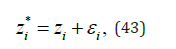
where varepsilon_i is a random variable. Noise is introduced only in the variable z, which corresponds to the experimental situation in which the frequency is prescribed and the spatial parameter is determined by measurement. In the illustrations, a moderate number of points is used, sufficient for visual control of branch geometry without overloading the figure.

Recognition algorithm. Branch recognition is performed by an iterative residual-minimization method. At each iteration, the set of points is divided into two subsets, each branch is approximated by an equation of a central second-order curve using approaches to conic fitting [11], the points are redistributed according to the minimum-residual criterion

and the procedure is repeated until the partition stabilizes.

The mean residual

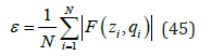
and the fraction of correctly classified points

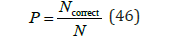
are used to estimate accuracy. These metrics make it possible to distinguish stable and ill-conditioned branch configurations; numerical stability issues in fitting circles and ellipses are discussed in detail in works on least-squares fitting of conic sections [12].

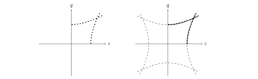
Graphical notation. In the figures, points represent a synthetic sample in the first quadrant. Solid parts of the curves show the physically observable part of the branch corresponding to z≥0, q≥0. Dashed curves show the central continuation of the same secondorder curve into the other quadrants (Figure 1).

Figure 1:Unlabeled points.

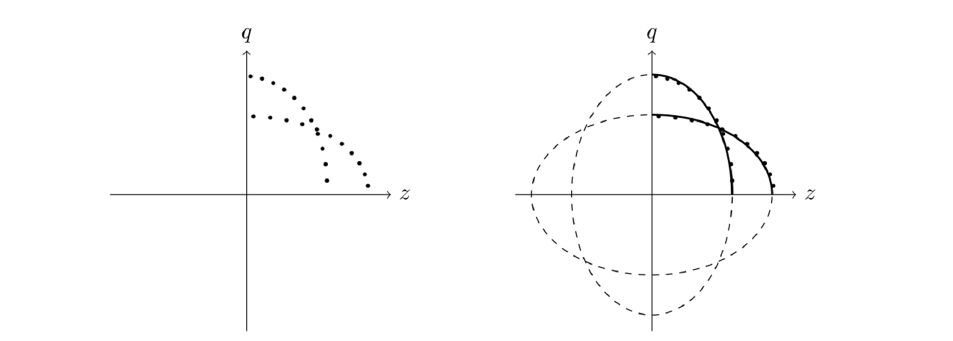
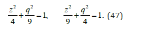
Two elliptic branches. The first test corresponds to two central elliptic branches

Recognition is stable: the branches have different orientations of the semi-axes and intersect only locally. Classification errors are localized near the intersection points (Figure 2).

Figure 2:Unlabeled points.

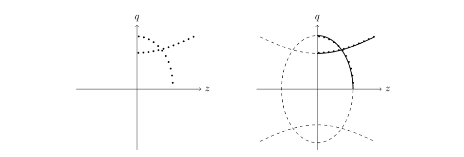
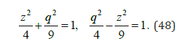
Elliptic and hyperbolic branches. The second test is defined by the system

The branches differ topologically: the elliptic branch is closed, whereas the hyperbolic branch is unbounded. Therefore, classification is the most stable in this case and requires the minimum number of iterations (Figure 3).

Figure 3:Unlabeled points.

Two hyperbolic branches. The third test is defined by

This case is more difficult than recognition of elliptic and hyperbolic branches because both branches are open. Nevertheless, the difference in opening directions provides stable separation (Figure 4).

Figure 4:Nearly coincident ellipses.

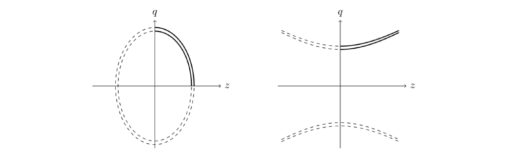
Nearly indistinguishable branches. The fourth test is used to demonstrate the boundary of applicability of the method:

These branches have close semi-axes and a small visible gap, which makes classification sensitive to noise. The fifth test is defined by

Here the branches have close asymptotes and slightly different focal parameters.

Result of the numerical experiment. In the first three tests, the algorithm stably separates the sample into two central secondorder curves. In the last two cases, the problem becomes illconditioned: the fraction of correctly classified points depends substantially on the noise level and the initial partition. Thus, the numerical experiment not only confirms the operability of the method but also reveals the natural boundary of its applicability.

Discussion of Results

The numerical experiment shows that the stability of spectral branch recognition is determined not only by the noise level but, first of all, by the geometry of the branches themselves in the space (z,q).

The most stable case is the joint recognition of elliptic and hyperbolic branches. This is because the corresponding secondorder curves have different topological structures: an elliptic branch is closed, whereas a hyperbolic branch is open. As a result, the local regions of minimum residual are well separated, and the iterative point-redistribution procedure stabilizes rapidly.

Recognition of two elliptic branches is more sensitive to noise. In this case, both branches have the same topology and differ mainly in the ratio of their semi-axes. When the distance between the branches is small, sample points near the intersection may belong to different local minima of the residual functional. This deteriorates the conditioning of the classification problem.

The case of two hyperbolic branches occupies an intermediate position. Although both branches are open, the difference in their opening directions creates a stable global separation of the data. However, when the asymptotes are close, the problem again becomes ill-conditioned.

The case of nearly indistinguishable branches is especially important. For close ellipses and hyperbolas, a small change in curve parameters leads to a significant change in the classification result. This means that recovering operator parameters is highly sensitive to experimental errors in regions of spectral proximity.

Thus, the geometric proximity of branches is directly related to the conditioning of the inverse problem. The smaller the distance between the branches in the space (z,q), the higher the sensitivity of model-parameter recovery to noise and the less stable the data partition becomes.

The obtained result has an important physical interpretation. Close branches correspond to modes with close spatial-frequency characteristics. In this case, the system becomes spectrally weakly distinguishable, and the experimental data are insufficient for reliable separation of the modes without additional a priori information.

It should be emphasized that only reversible conservative systems have been considered in the present paper. In this formulation, the characteristic equation contains only even powers of the parameters λ and ω. This leads to a central structure of spectral branches in the space (z,q). However, the absence of the mixed term zq requires additional symmetries of the operator and is not a direct consequence of reversibility alone. In dissipative and nonsymmetric systems, mixed and odd terms may appear, leading to displacement and rotation of the branches.

From a practical point of view, the proposed approach can be considered as a basis for constructing libraries of spectral images of materials. In this case, operator parameters are determined not directly from the coefficients of the differential equation but through the geometry of the observed spectrum. Such a formulation opens the possibility of machine recognition of materials and structures from their spatial-frequency characteristics.

Thus, the geometry of the branches of the dispersion curve can be regarded as a direct manifestation of the structure of the operator. In this formulation, the inverse identification problem is reduced to recognition of the geometric parameters of spectral branches.

Conclusion

The paper proposes an approach to identifying the parameters of a dynamic model of a gradient porous beam based on analysis of spectral geometry. It is shown that the transition from k(ω) to the full spatial parameter λ(ω) makes it possible to take into account wave, boundary, and scale components of the solution simultaneously.

The main result of the paper is the following theorem.

Theorem. Identification of the parameters of a linear conservative dynamic system with two independent kinematic variables, whose characteristic equation in the variables z=λ² and q=ω² is quadratic with respect to q, is equivalent to recognizing two central second-order curves of the equation F(z,q)=0 from the experimentally recovered dependence λ(ω); under additional symmetries of the operator, these curves have an axial form without the mixed term zq. Theorem

Proof. In the harmonic regime, the solution is sought in the form

Substitution of representation (52) into the equations of motion leads to a homogeneous algebraic system for the amplitudes A and B. A nontrivial solution exists if and only if the determinant of this system is zero:

F (λ,ω ) = 0. (53)

Since the system is conservative and reversible, the frequency enters through ω², while the spatial parameter enters through even powers of λ. Therefore, the variables

z = λ ² , q =ω²

are introduced. In these variables, the characteristic equation takes the form

F (z, q) = 0. (55)

Reversibility excludes linear terms in z and q, and therefore each branch in the plane (z,q) has the central form

Here the coefficients a, b, c, and d denote the coefficients of the approximating second-order curve and are not related to the coefficients of the characteristic equation.

In the absence of gyroscopic and other nonsymmetric couplings, additional symmetries of the operator exclude rotation of the branches, that is, the mixed term zq. Then the central secondorder curve takes the axial form

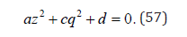
By the assumption of the theorem, equation (55) is quadratic with respect to q:

Consequently, the solution set splits into two branches

The experimentally recovered values λ_i=λ(ωi) define points 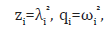, which must belong to one of the two branches up to experimental error. Therefore, recovery of the model parameters is reduced to determining the coefficients of the equation F(z,q)=0 and partitioning the experimental points between the two branches q₁(z) and q₂(z). The theorem is proved.

The obtained result shows that the inverse problem can be formulated as a problem of geometric recognition of spectral branches. This approach is applicable to a broad class of systems described by equations of the form F(λ,ω)=0, including gradient and defective media.

Promising directions for further research include accounting for dissipative effects, extending the approach to multimode signals and to two- and three-dimensional problems, and constructing libraries of reference spectral structures for machine recognition of materials.

References

1. Mindlin RD (1964) Micro-structure in linear elasticity. Archive for Rational Mechanics and Analysis 16: 51-78.
2. Toupin RA (1962) Elastic materials with couple-stresses. Archive for Rational Mechanics and Analysis 11: 385-414.
3. Askes H, Aifantis EC (2011) Gradient elasticity in statics and dynamics: An overview of formulations, length scale identification procedures, finite element implementations and new results. International Journal of Solids and Structures 48: 1962-1990.
4. Cowin SC, Nunziato JW (1983) Linear elastic materials with voids. Journal of Elasticity 13: 125-147.
5. Belov PA, Lurye SA (2014) Mathematical theory of defective media. Palmarium Academic Publishing, Russia, p. 336.
6. Egorova MS, Kalyagin MYu, Rabinskiy LN (2025) Theory of rods (plates) formulated for non-classical models of porous media in the mechanics of deformable bodies. Proceedings of MAI 142.
7. Graff KF (1991) Wave motion in elastic solids. Dover, New York, USA.
8. Mead DJ (1996) Wave propagation in continuous periodic structures. Journal of Sound and Vibration 190: 495-524.
9. Gantmacher FR (1967) The theory of matrices. Nauka, Moscow, Russia.
10. Gladwell GML (2004) Inverse problems in vibration. (2^nd edn), Kluwer Academic Publishers, Dordrecht, Netherlands.
11. Fitzgibbon A, Pilu M, Fisher RB (1999) Direct least squares fitting of ellipses. IEEE Transactions on Pattern Analysis and Machine Intelligence 21: 476-480.
12. Chernov N, Lesort C (2005) Least squares fitting of circles and ellipses. Journal of Mathematical Imaging and Vision 23: 239-252.