Research on the Grid Construction Method of Multibeam Non-Tide-Gauging Vertical Datum Based on Optimized Xgm2019 Gravity Field Model

Multibeam sounding serves as the predominant technique for marine bathymetric surveying at present. Conventional multibeam bathymetry requires the deployment of tide gauge stations to implement water level correction. The multibeam non-tide gauging mode developed in recent decades eliminates manual tide observation procedures. Numerous domestic and international studies and engineering practices have verified that GNSS-based multibeam non-tide gauging survey can significantly promote sounding ac-curacy and operational efficiency [1-3]. Existing scholarly research mainly focuses on experimental verification of non-tide bathymetry with single tide gauge stations and single beam systems. For multibeam non-tide water level correction over large-scale sea areas, single-station correction using the geodetic height of chart datum from an individual tide gauge is acceptable when the required sounding precision is relatively loose. In contrast, the multi-tide-gauge mode demands establishing a regional geodetic height grid model of chart datum (HDM) by analyzing the mutual relationships among multiple vertical reference surfaces including mean sea level, quasi-geoid, chart datum and reference ellipsoid. The refinement of the quasi-geoid is the core procedure for constructing the above grid model, which realizes the elevation conversion between geodetic height and normal height via global gravity field models. This paper adopts the widely recognized optimized XGM2019 gravity field model and carries out targeted research and experimental verification on the methodology and workflow for generating the geodetic height grid model of chart datum with Surfer software and elevation anomaly calculation programs.

XGM2019 gravity field optimization model

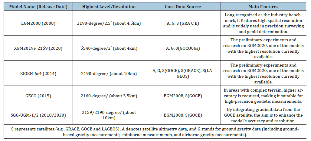
As the experimental version of EGM2020, XGM2019 was released by the Institute for Astronomy and Physical Geodesy at the Technical University of Munich in 2019, with its upgraded or optimized version published by ICGEM (International Centre for Global Gravity Field Models) in 2020. XGM2019e_2159 represents a global gravity field model of the same order as EGM2008, achieving a full order of 5399 (with spherical harmonic coefficients extended to order 5540). Its data sources include the GOCO06s satellite model, short-wavelength ground gravity measurements, land and ocean gravity anomalies provided by NGA identical to those of XGM2016 and EARTH2014 terrain gravity data for land surfaces. XGM2019e_2159 is recognized as offering greater consistency globally and operating independently of existing high-resolution global models, particularly demonstrating enhanced performance over oceans [4-7]. Comparison of parameters with main-stream global gravity field models is presented in Table 1. The study employs the Guangdong Province XGM2019e_0.005° model as the optimized XGM2019 gravity field, which was developed using the “Removal-Fitting-Recovery” method and integrating data from digital terrain models, ground gravity observations, Earth’s gravity field models and GPS levelling measurements to establish a regional quasigloboidal surface model with a ground resolution of 0.3′ (ap-proximately 0.6 km).

Table 1:Global Gravity Field Model Parameter Table.

Principles of grid model (HDM) construction

Figure 1:Schematic diagram illustrating the relationships between various reference surfaces in model construction.

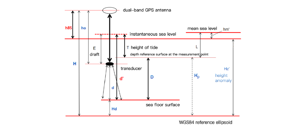
The key to tidal depth measurement technology lies in establishing a separation model between the depth reference surface and the reference ellipsoid. The relevant reference surfaces involved include: the multi-year average sea level, the depth reference surface, the reference ellipsoid and the 1985 national elevation reference surface, as shown in Figure 1. H′_Z represents the difference between the WGS84 reference ellipsoid surface and the 1985 national elevation datum, i.e., the elevation anomaly; h ′_m denotes the local multi-year average sea level difference relative to the 1985 national elevation datum; L is the depth reference surface value. The local multi-year average sea level can be determined through long-term tide observations at monitoring stations, or via levelling surveys and analysis of the relationship between the quasi-geoid surface and the average sea level at adjacent tide gauge stations. The difference between the regional multi-year average sea level and the geoid surface is termed sea surface topography, which is generally consistent across large areas. The depth reference surface height is measured relative to the average sea level; when con-structing a regional depth reference surface model, spatial interpolation is applied to L-values obtained from discrete tide gauge stations to generate a continuous, unified depth reference surface grid. Elevation anomalies H ′_Z are calculated using the XGM2019e gravity field model at a 0.005°×0.005° grid resolution and corrected based on measured elevation values acquired via GNSS levelling at known points. In summary, the formula for calculating the geodetic elevation H ′_P of the depth reference surface at any point within the marine survey area is as follows:

Construction process of the grid model (HDM)

The specific procedure for constructing a high-precision geodetic elevation grid model (HDM) of the depth reference surface by utilizing data from multiple known tide gauge stations in the survey area is as follows:

A. Use Surfer software to create a regular grid file for the survey area, define grid spacing and generate the depth reference surface grid model by applying Inverse Distance-Weighted Interpolation (IDW) using the known L-values of each tide gauge station’s depth reference surface.
B. Calculate the elevation anomaly value H′_Z at each grid centre point using the gravity field model’s elevation anomaly calculation program.
C. For each tide gauge station h ′_m , derive a grid model representing the multi-year average difference between sea level and the 1985 national elevation reference using in-verse distance- weighted interpolation;
D. Finally, determine the geodetic elevation values of each grid centre point based on Equation (1), thereby constructing a grid model without tidal water level corrections.

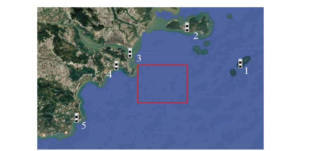
The survey area is located in Guang’ao Bay, Shantou City, Guangdong Province, as indicated by the red box in Figure 2. To implement tidal control across the entire survey zone, five tide gauge stations have been established: Stations 1 and 3 are temporary stations, while Stations 2, 4 and 5 are permanent stations. Data from the reference surface have been collected at the permanent stations; synchronization between the temporary and permanent stations enables the determination of the local mean sea level and theoretical depth reference surface. All five stations have undergone joint levelling measurements with high-grade levelling points to verify the accuracy of mean sea level calculations.

Figure 2:Location of the Guang’ao Bay survey area and tide monitoring station.

Grid Construction

The first step involves importing the latitude/longitude coordinates and L-values of the depth reference surface from five tide gauge stations into Surfer software as standard files to generate a depth reference surface grid model. This approach employs the inverse- distance-weighted multi-station tidal correction method [8], which operates on the principle that a point’s tide level is proportional to its distance from the tide gauge station: stations farther away exert less influence on the local tide level and vice versa. Select “Gridding Method” → “Inverse Distance to a power” in the Surfer menu, then set a square grid spacing of 0.005° for both latitude and longitude to create the grid model (Figure 3-4), while generating an output text file in L-XYZ format. The second step requires launching the gravity field model elevation anomaly calculation program and importing the XGM2019e_0.005° gravity field model. Import the *.XYZ text file generated in the first step as input data, setting the elevation anomaly correction method to “contour method” as illustrated in Figure 5. The program outputs the elevation anomaly values at each grid center point.

Figure 3:Surfer software generates a grid.

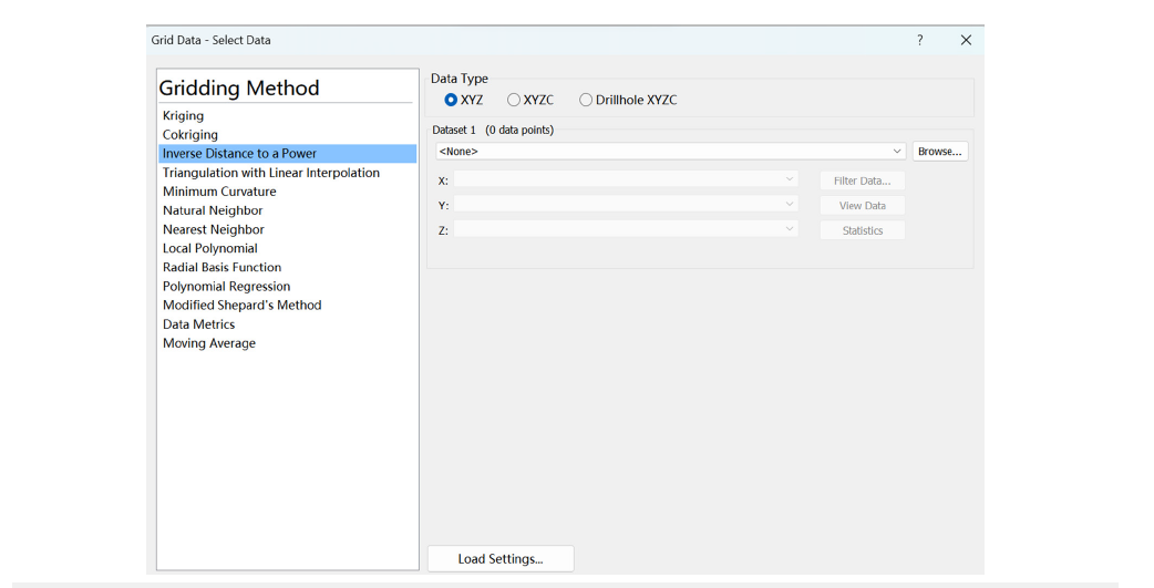
Figure 4:Deep reference plane grid 3D model.

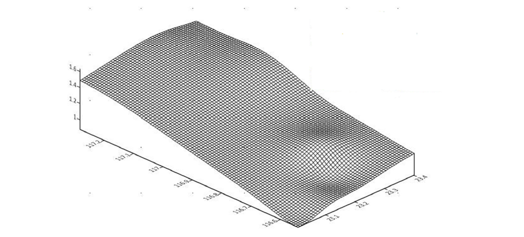
Figure 5:Program for calculating elevation anomalies in gravity field models.

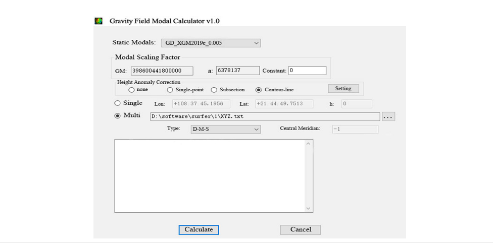
The “Elevation anomaly correction” function is used to generate elevation anomaly correction values. This step is crucial for improving the accuracy of the quasi-geoid sur-face and includes three methods: single-point, segment-based and contour-line methods:

A. Single-point correction method. This method directly uses the elevation anomaly data from measured individual points to calibrate the gravity field model, obtain correction coefficients and then apply point-by-point adjustments to the model-derived elevation anomalies; it is suitable for scenarios with sparse point distributions or local refinement requirements.
B. Segment-based correction method. This approach divides the survey area into segments, statistically analyzes the elevation anomalies of known points within each grid segment, calculates systematic deviations between the model and measured values, de-rives segment-specific correction parameters through polynomial fitting and finally ap-plies these parameters to adjust elevation anomalies in the corresponding grids; it is applicable when terrain variations within the survey area are moderate, where using a small number of known points and applying polynomial quadratic surface fitting yields satisfactory results [9].

To use this method, the number of known points must exceed 4. Derive expressions for elevation anomalies ξ_i (i = 1,2,3..., n) in terms of coordinate values and based on the quadratic surface model, derive n error equations for the elevation anomalies:

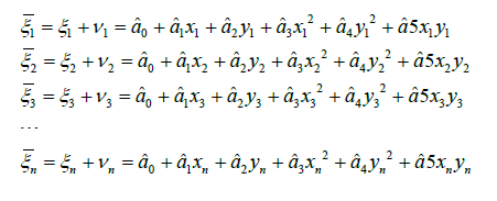
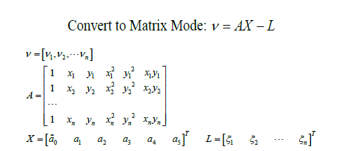
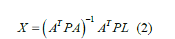
Using the least squares method and following Principle, V^T PV = min the coefficient aˆ_i can be determined, as expressed below:

C. Contour Line Method Correction. The contour line method performs spatial interpolation using elevation anomaly contour maps and is suitable for survey areas with a relatively uniform distribution of known points. The steps include: Plotting the elevation anomaly values of known points onto a map or digital grid, then drawing contour lines at 1-5 cm intervals; subsequently applying Kringing interpolation to un surveyed points using these contour maps to obtain elevation anomaly correction values; finally overlaying the interpolation results with the gravity field model for adjustment. This method reflects spatial continuity of anomalies, with accuracy depending on contour density and interpolation algorithm. The Kringing interpolation algorithm determines the elevation of the target point by analyzing its relative spatial relationship to nearby known points and employing a linear unbiased optimal estimation [10]. The formula is as follows:

In the formula: λ_i is a weighting factor that represents the influence of known points on the value of the unknown point. Certain constraints must be satisfied during interpolation:

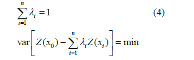
Two constraints are applied: The sum of weights must equal 1 and the estimated variance must be minimized. Under these conditions, the weight coefficients can be deter-mined, after which the elevation of the target point is calculated using Formula (3). Comprehensive Application and Considerations: In practical applications, the method should be selected based on data distribution and accuracy requirements. Accuracy verification requires establishing independent reference points and evaluating performance through mean deviation errors [10]. Additionally, coordinate system consistency, DEM resolution and gravity field model selection (e.g., type) significantly impact correction accuracy; parameters should be adjusted according to regional geological characteristics.

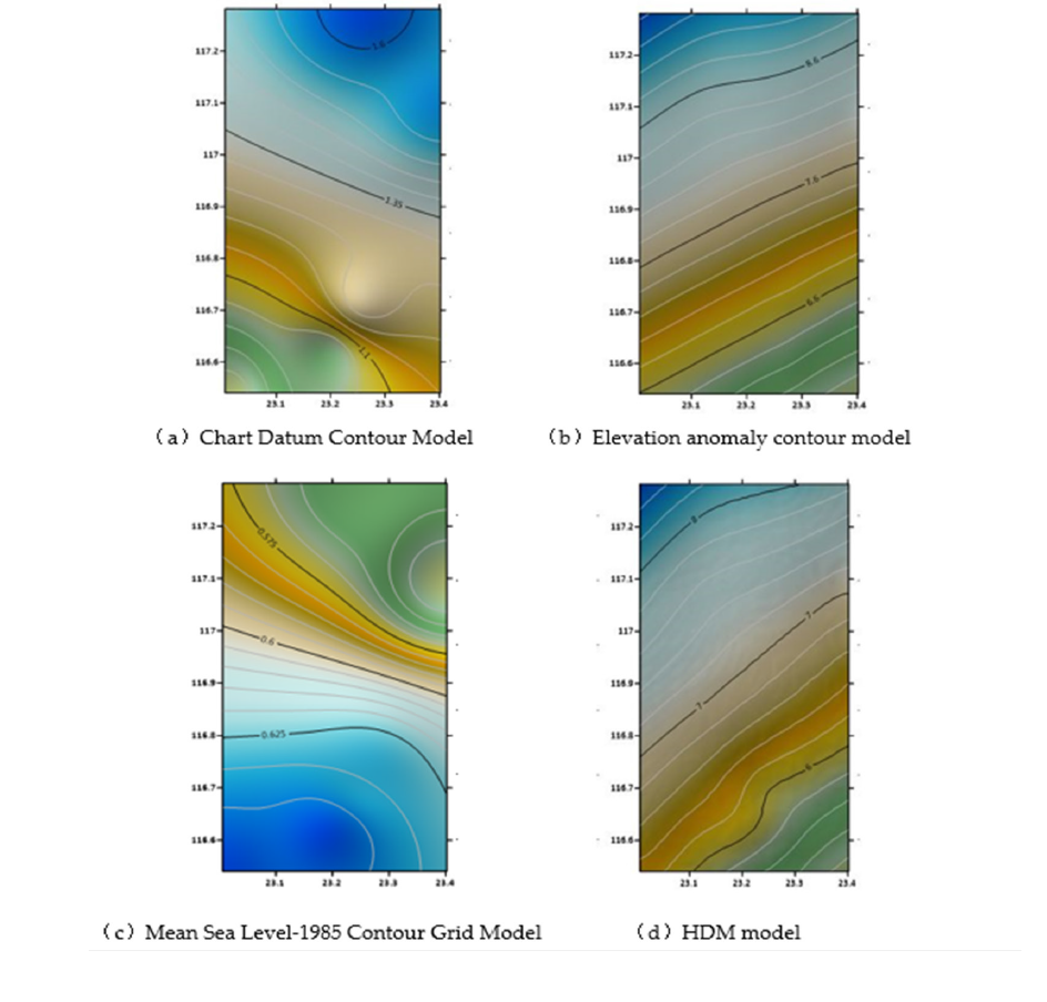
The third step: Import the coordinates of five tide gauge stations and the multi-year average sea surface elevations relative to the 1985 national elevation datum into Surfer software as standard files, then generate a grid model using Inverse Distance Weighting Interpolation (IDW). The fourth step: After establishing the depth reference surface, elevation anomalies and the multi-year average sea surface-1985 grid model, calculate the geodetic elevations at each grid center point using Formula (1) to produce the depth reference surface geodetic elevation grid model (HDM). The process is illustrated in Figure 6, with the final output being an HDM-XYZ text file.

Figure 6:Flowchart of the grid construction steps.

Water level correction

The multi-beam uncalibrated tide level correction using the Deep Reference Surface Geoid Grid Model (HDM) is performed as follows:

Open the Caris 11.3 multi-beam data processing software. After importing the raw survey line data, select “Auxiliary Data” → “ASCII”. This ASCII file contains GPS date, UTC date, local time, latitude and longitude and geodetic elevation values, which will re-place the original multi-beam depth measurements. Upon completion of this replacement, the displayed water depth reflects the seabed topographic geodetic elevation values.

Open “Georeference Bathymetry” (geographic registration of depth data), select the “GPS Tide” mode and in the parameter settings section: choose “Model File” as HDM-XYZ and “ASCII Format Information File” as the corresponding*.info file containing the geodetic elevation grid model data serving as the depth reference for multi-station correction; refer to the relevant manual for specific file format details.

Click “OK” to apply the water level correction.

Accuracy verification

The accuracy verification of the results comprises three components: First, comparing the accuracy of the XGM2019e_0.005° gravity field model with three other models within the Guangdong survey area; second, evaluating the accuracy of the correction function in the elevation anomaly calculation program using known GNSS leveling measurements; third, comparing water depth accuracy between conventional manual tide monitoring and unmonitored conditions. The detailed procedures are as follows：
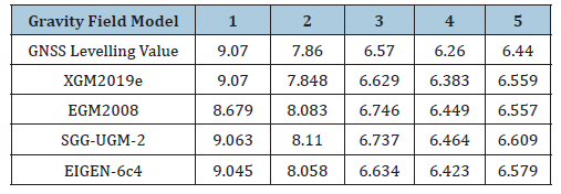
A. Substitute XGM2019e_0.005°, EGM2008, SGG-UGM-2 and EIGEN- 6c4 respectively into the elevation anomaly calculation program to obtain model-derived values for five known tide gauge stations. As shown in Table 2, the model values generated from XGM2019e_0.005° are closer to the actual GNSS leveling measurements in the Guang-dong survey area.

Table 2:Comparison of measured values with program- generated values Unit (m).

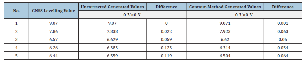
B. Using the “Elevation anomaly correction” function in the elevation anomaly calculation program, the internal accuracy was evaluated using data from five known tide gauge stations to compare deviations between GNSS-level measured values and those generated by the “uncorrected” and “contour method” approaches; details are shown in Table 3. The deviation between the model’s “uncorrected” values and actual measurements ranges from 0 to 15cm, while that between corrected values and actual measurements ranges from 0 to 6cm. Thus, the “elevation anomaly correction” function enhances the accuracy of elevation anomaly values produced by the gravity field model.

Table 3:Comparison between measured values and program-generated values Unit (m).

C. To verify the external agreement accuracy of the HDM model without tide verification correction, three areas (A, B and C; Figure 7) within the survey zone were selected for traditional single-station (Tide gauge station 3), dual-station (Tide gauge stations 4 and 5) and multi-station water level correction (Tide gauge stations 1-5) analyses, respectively. The results were then compared with those obtained using the tide-free method; the com-parisons are shown in Figures 8a-8c.

Figure 7:Schematic diagram of comparison areas A, B and C.

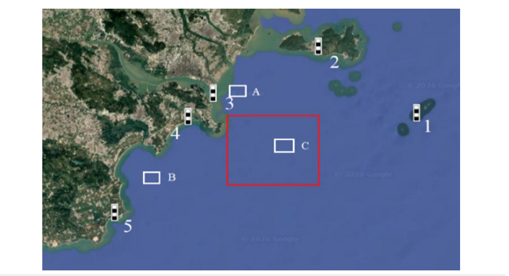
Figure 8:Figure of comparison results for two tide gauging modes.

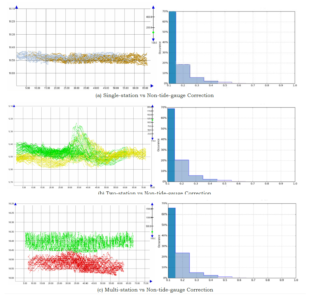
D. The comparison between the two tide verification modes was conducted using the calculation of cross-point depth discrepancy values. Figure 8 illustrates the comparison results, with (a) to (c) representing single-station correction versus no-tide-verification comparison, dual-station correction versus no-tide-verification comparison and multi station correction versus no-tide-verification comparison respectively. The left panel shows a screenshot from the sub-region editing module of Caris software, while the right panel displays the corresponding column chart of cross-point depth discrepancy statis- tics. As shown in the comparison data charts (a)-(c), within the 20-30 m water depth range, 100% of depth discrepancies remain within 0.5m and approximately 70% are controlled below 0.1m. These results comply with the depth discrepancy tolerance requirements specified in GB12327-2022 “Specifications for Hydrographic Surveys”. The sub-region editing module screenshots demonstrate that the differences between correction values for both verification modes along the same survey line progressively increase, with standard deviations of 0.093m, 0.109m and 0.124m, respectively. Three primary factors contribute to increased cross-point depth discrepancies: first, the distance from the verification stations in the comparison area; second, the growing uncertainty in station data due to wave effects and dynamic draft variations when transitioning from single to multi-station measurements; third, the use of an interpolation model for the vertical reference grid in no-tide-verification methods, where interpolation values approach actual measurements closer to verification stations and decrease in accuracy with greater distance.

The non-tide-gauge sounding mode can markedly improve the operational efficiency and data accuracy of bathymetric surveying, possessing great practical value in engineering applications. In this paper, a method for constructing the vertical datum grid for multibeam surveys without tide gauge observations is investigated using field data acquired in the Shantou Sea area of Guangdong Province. Experimental results reveal that the XGM2019e_0.005° ultra-high-degree gravity field model effectively improves the precision of regional vertical datum grids and meets the practical demands of hydrographic surveys along the Guangdong coast. As CARIS software does not supply standardized operating workflows for multi-station water level correction under the non-tide-gauge mode, a complete technical processing scheme is proposed in this work. HDM modelling and accuracy verification prove that the internal and external coincidence accuracy of corrected data conforms to the specification standards, which verifies the reliability and strong practicability of the proposed method. Meanwhile, this study identifies prominent regional discrepancies in the precision of global gravity field models and no single model delivers optimal performance for all sea areas; accordingly, model selection should be optimized according to local marine conditions. Furthermore, global gravity field models suffer from low precision in offshore waters far from the mainland. Without constraint corrections from GNSS levelling measurements on surrounding islands and reefs, the reliability of grid interpolation outputs will be degraded. Future research can focus on the optimal matching of gravity field models for various sea zones and high-precision correction methods for offshore vertical datums, so as to further perfect the technical framework of high-precision multi-beam bathymetry based on the non-tide-gauge technique..

1. Feng Guozheng, Cao Lei, Ma Yaochang (2018) Uncalibrated tide-measuring depth measurement technology based on the EGM2008 model. Surveying and Mapping Science 43(1): 27-30.
2. Jiang Lin, Chen Zhenyu, Hu Yunpeng (2019) Application of multi-beam uncalibrated tide-measuring depth measurement technology based on the EGM model. Journal of Marine Technology 38(5): 104-108.
3. Wang Shuangxi, Miao Shiwei, Xu Jiakun (2016) Construction of vertical reference models for multi-beam uncalibrated tide-depth measurements. Marine Surveying and Mapping 36(1): 48-50.
4. Förste, Christoph, Bruinsma S, Abrikosov O (2014) EIGEN-6C4-The latest combined global gravity field model including GOCE data up to degree and order 1949 of GFZ Potsdam and GRGS Toulouse. AGU Fall Meeting Abstracts.
5. Zingerle P, Pail R, Gruber T (2020) The combined global gravity field model XGM2019e. Journal of Geodesy 94(7): 419-432.
6. Pavlis NK, Holmes SA, Kenyon SC (2012) The development and evaluation of the Earth Gravitational Model 2008 EGM2008. Journal of geophysical research: Solid Earth 117(B4).
7. Xu Lijun, Cheng Xinping (2022) Feasibility analysis of a multi-station tide level correction method based on distance reciprocal weighting. Journal of Wuhan University of Technology 46(4): 755-758.
8. Yu Xiaoping, Yang Guodong, Xu Huiping (2007) Research on converting GPS elevations to normal heights in strip-shaped regions. Journal of Jilin University (Earth Sciences Edition) 1:185-189.
9. Li Junhai, Wen Hanjiang, Fang Aiping (2011) Application of Kriging combined with least squares fitting in GPS elevation modeling. Surveying and Mapping Science 1: 99-101.
10. Zhao Jianhu, Liu Jingnan (2008) Multi-beam bathymetry and image data processing. Wuhan: Wuhan University Press, China.