Comprehensive Calibration Study on Multi-Beam Transducer Installation Deviations Based on Total Least Squares

The installation deviations of multibeam transducers exert a non-negligible impact on bathymetric accuracy, with calibration methods typically utilizing seabed data from specific terrains processed in a prescribed sequence. Godin (1996) established certain requirements for calibration line deployment and terrain selection in the Patch Test, pro-posing the following calibration sequence: Pitch deviation, yaw deviation and roll deviation. Prunus Salicina Jiabiao, based on the influence characteristics and interrelationships of these deviations, suggested an alternative sequence: roll deviation, yaw deviation and pitch deviation. Deng Weihong advocated for pitch deviation, roll deviation and yaw deviation calibration sequence. Currently, the most widely adopted calibration sequence in China is roll deviation, pitch deviation and yaw deviation. These varying processing sequences primarily aim to eliminate interference or coupling effects among different installation deviations of multibeam systems [1]. Regarding individual calibration, many researchers have proposed more precise algorithms building upon traditional calibration methods. For instance, to address in-complete roll deviation calibration of multibeam transducers, Zhang Zhiwei introduced a method estimating transducer roll deviation using approximate planes [2]. Sun Wenchuan developed a secondary roll deviation calibration method based on weighted least squares [3], while Liu Guoqing proposed an iterative roll deviation algorithm accounting for acoustic ray bending [4]. However, separate calibration inherently severs the interconnections among various deviations, neglecting their mutual influences. Consequently, even under stringent calibration conditions, achieving high calibration accuracy remains challenging.

In contrast, integrated calibration methods fully consider the coupled relationships among deviations, enabling simultaneous estimation of all deviation parameters through a unified model. The calibration process involves: First completing survey operations on all lines within the calibration area, treating the obtained measurements as observations, then combining them with prior information about seabed topography to solve all deviation parameters jointly according to an optimal criterion (e.g., least squares) [5]. International scholars have conducted in-depth research in this area. Dunnewold (1998) calculated all parameter values using an integrated model based on least squares, assuming known shape and absolute position of a seabed object. Riley (2000) employed stochastic optimization to calibrate four parameters of multibeam bathymetric systems simultaneously. Nicolas Seube et al. [6] proposed using MIBAC (Multibeam-IMU Boresight Automatic Calibration) for comprehensive installation deviation detection. In the observation models constructed by integrated calibration methods, the observation equation consists of water depth measurements on one side and the deviation parameters to be estimated with their corresponding coefficients on the other. Most existing studies employ traditional least squares, which implicitly assumes that observations contain errors while coefficients are error-free. For this problem, water depth as a measured value undoubtedly contains errors, but the coefficients derived from navigation data (including positioning and attitude) inevitably possess errors (particularly attitude errors). Clearly, this problem exhibits distinct Error-In-Variable (EIV) characteristics. Accounting for these characteristics, the appropriate solution should be the Total Least Squares (TLS) solution. This paper investigates transducer installation deviation calibration within the more realistic EIV/TLS framework.

In the classical least squares adjustment model, it is only assumed that the observation vector contains random errors, while the coefficient matrix is known and non-random. However, in many practical problems such as digital terrain model fitting, geodetic inversion, GIS spatial data analysis, landslide monitoring and coordinate trans-formation, both the observation vector and the coefficient matrix describing the functional model are composed of observational data and both contain random errors. Such adjustment models are referred to as EIV (Errors-In-Variables) models [7-9], with the specific form as follows:

In the equation, L represents the observation vector of n×1 , ΔL is the random error vector contained in the observation vector, A represents an n×mcoefficient matrix containing n×m random errors Δ_A , e_A = vecΔ_A e_A is the nm×1-dimensional vector obtained by column-vectorizing Δ_A ; X is the parameter vector to be estimated for m×1.

Since the classical least squares method only considers errors in the observation vector, while the EIV model’s coefficient matrix contains errors, the classical least squares estimation method is no longer applicable [10]. To address the problem where both the coefficient matrix and observation vector have errors, the least squares estimation criterion needs to be generalized and extended. This involves minimizing the sum of squared residuals for all observational data (including both the observation vector and coefficient matrix), which is known as total least squares [11]. The basic idea of total least squares can be summarized as follows: Not only does the observed quantity L contain observation errors ΔL , but the coefficient matrix A also has errors Δ_A . In total least squares, the solution to the linear equation (1) is considered [12]. For the sake of facilitating problem discussion, let the mean vector and covariance matrix of the error vector be

In the formula, ⊗ represents the Kronecker product of matrices, I_n and I_m are identity matrices of orders n and m respectively, is the unit weight variance, Σ_L and Σ_A are the covariance matrices of the observations and coefficient matrix respectively.

Obviously, equation (1) can also be rewritten as

The total least squares method for solving the above equation can be formulated as a constrained problem:

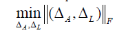
The constraint is , where is the Frobenius norm of the matrix, which is defined as the square root of the sum of the squares of all elements in the matrix.

Establishment of coordinate systems and determination of parameters

The calibration of transducer installation deviations involves the definition of coordinate systems and the definition of transformation parameters between coordinate systems. For convenient representation, the following three sets of righthanded rectangular coordinate systems are established: The local horizontal coordinate system, abbreviated as the l-system (local), with a reference point on the horizontal plane as the origin and the three axes pointing north-east-down, serving as the reference coordinate system for navigation and positioning; the body coordinate system, abbreviated as the b-system (body), with the centre of the navigation module as the origin and the three axes pointing for-ward-right-down relative to the measurement vessel carrier; the multibeam sonar coordinate system, abbreviated as the m-system (multi-beam). The multibeam sonar coordinate system is rigidly connected to the vessel body. During installation, it is intended to align with the b-system, but due to installation errors, there is an offset between them. The origin is the beam emission point of the multibeam sonar, the z-axis points vertically downward, the multibeam fan lies within the yoz plane, the positive direction of the y-axis points to-ward the starboard side of the vessel and the x-axis forms a right-handed system with the y and z axes.

As mentioned earlier, this paper adopts the feature target matching idea of Dunne-wold. That is, a body of water is selected where there are targets with distinct features and known three-dimensional positions (horizontal position and depth). Measurement operations are conducted in this sea area and the measured values obtained from these operations are matched to the known target positions using a certain matching method. The observations include the following data: position data measured by the navigation module, known target position data, attitude data measured by the navigation module, preset beam angle data and beam-measured distance (determined by the time difference of measurement).

Traditional single-item calibration compares seabed topography derived from two calibration survey lines and does not involve the absolute position of seabed target points in the local horizontal coordinate system; thus, it only calibrates the angular installation deviations of the transducer. In contrast, comprehensive calibration requires comparing the known position information and measured information of target points and then determining the installation deviation values using total least squares adjustment. During coordinate transformation, there are not only angular installation deviations between the transducer and the survey vessel but also distance deviations between the transducer’s depth-measuring centre and the vessel’s navigation positioning centre. Since this deviation cannot be measured accurately, it is treated as an unknown parameter in the comprehensive calibration model of this paper. The installation deviations of the transducer are denoted by OC (offset coefficients), the distance deviations by the vector matrix TOC (translational offset coefficients) and the angular deviations by the rotation matrix ROC (rotational offset coefficients). From the coordinate system definitions above: the vector from the origin of system l to any point is expressed in system l as the coordinates of that point, such as the coordinates of the origin of system b measured by the navigation module. The vector from system b to system m is TOC and the rotation of system m relative to system b is ROC, which are the quantities to be determined during OC calibration.

Establishment and solution of function models

Let the position vector of the target be , where the subscript denotes the vector from the origin of coordinate system l to target t and the superscript denotes the coordinates of this vector in system l ; follow the same convention hereafter. Let the position of the measurement ship’s body be . Let TOC be . Let the attitude matrix of the carrier be , which is specifically a direction cosine matrix and serves to convert the coordinates of a vector in the b -system to the coordinates of that vector in the l -system. Similarly, ROC is expressed as . Let the beam opening angle be θ and the beam ranging be s . Based on the above definitions, the following functional relationships hold:

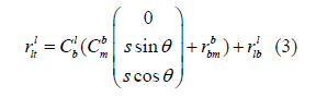
For the sake of representation, 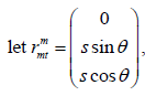then we have

In the formula , is the transpose of . Since is a rotation matrix 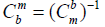and similarly for others.

In equation (5) is determined by s (distance measurement) and θ (beam opening angle). Among these, s contains measurement error s due to inaccuracies in sound speed and sound ray, etc. θ is the set angle, which can be considered as having no error or its error can be absorbed by as the target position, is assumed to be known. needs to be measured by the navigation module and contains measurement error. is TOC, which is the unknown to be solved. is the attitude matrix (transpose), which needs to be measured by the navigation module and contains measurement error. is ROC (transpose), which is the unknown to be solved.

In the traditional least squares method, it is assumed that only the left-hand side of (5) contains errors, which is clearly not in line with reality. To address this, equation (4) is re-arranged again as follows:

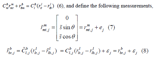
In the equation, j =1,2,----J , represents the j -th measurement e_i and ε_i denote the measurement error vector of the water depth point and the calculation error vector caused by navigation positioning and attitude measurement errors, respectively. Substituting equations (7) and (8) into equation (6), we obtain

Based on total least squares, let the cost function be the weighted sum of squared measurement errors, that is

Here, P_j and Q_j are the covariance matrices of e_j and ε_j , respectively. For simplicity in calculation, we assume that

Here, I₃ is a 3-dimensional identity matrix. Thus, the problem becomes a minimization problem that satisfies constraint (10) given in equation (9) and of course must also satisfy the properties of a rotation matrix. Introducing the 3×1-degree vector Lagrange multiplier C, we construct the following Lagrange function

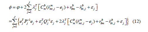
According to the minimized first-order necessity condition, we have

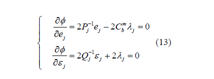
Substituting (14) into equation (9) yields:

Substituting equation (16) into equation (14), we obtain:

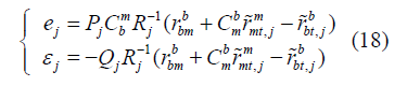
Substituting equation (18) into equation (10), we obtain:

Equation (19) has a concise form, namely the weighted sum of squares form. Based on the first-order necessity condition for minimizing Equation (19), we have

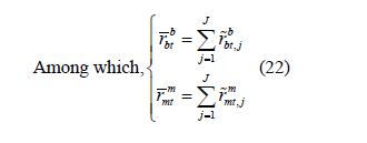
Substituting equation (21) into equation (19) yields:

Expanding equation (23) and considering the structure shown in equation (17), we obtain

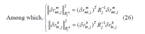
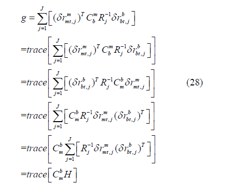
Since the first two terms on the right side of equation (25) are independent, minimizing equation (25) is equivalent to maximizing the following function

Since the trace of a scalar equals the scalar itself, is the product of a constant and the identity matrix and the matrices involved in the trace calculation are commutative [13], therefore:

Performing SVD decomposition yields :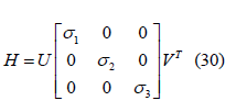

Substituting it into equation (28) and again utilizing the rotational property of trace operations, we obtain

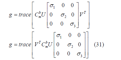
To maximize the above expression while considering that

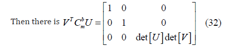
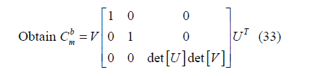
Notably, the equation uses det[U]det[V ] instead of 1 to ensure 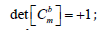; otherwise, might occur. In such a case, no longer represents rotation but rather a mirror-symmetric transformation [14]. This yields the rotor alignment deviation ROC; further decomposition yields individual deviation angles Substituting equation (33) into equation (21) allows determination of the distance installation deviation TOC.

To verify the effectiveness of the proposed algorithm, obstacle detection data from a specific measurement site near Beihai in Guangxi Province were selected for analysis. During field measurements, instrument installation parameters were calibrated by utilizing specialized underwater topography in designated areas; calibration parameters were calculated using the Caris parameter calibration tool in office processing; no time delay correction was required as the system employed a 1pps time synchronization signal. Parameter measurements were conducted sequentially for yaw deviation, pitch deviation and roll deviation, with the resulting multi-beam transducer installation deviations presented in Table 1.

Table 1:Parameters for converter installation deviation

The comprehensive calibration model proposed in this paper is based on accurate information of known seabed feature points. Due to constraints imposed by measurement conditions and data accuracy, the seabed topography -after undergoing traditional installation deviation calibration and various conventional corrections-is temporarily treated as the known reference; the seabed without installation deviation compensation is considered the measured seabed. Since seabed feature points are not obscured by installation deviations, the Caris data processing software utilizes these feature points to correlate known parameters (position and water depth) with observational data. Additionally, various datasets required for model fitting are obtained from multi-beam survey line analysis software and incorporated into the aforementioned model to calculate transducer installation deviations.

Using the field plot interface for calibration survey lines in the Caris processing software, users can select seabed topographic feature points and obtain related information such as location and water depth. Through the sub-area editing module and analysis methods, original measurement data for these feature pointsincluding ship attitude, beam angle and echo time-can be retrieved.

In the aforementioned model, for simplicity in derivation, the covariance matrices of the two measurement errors are treated as products of a constant coefficient ξ , ζ and an identity matrix. In this experiment, we set ξ =ζ =1 and define J = 6 as having 6 feature points; detailed information about these feature points is presented in Table 2 and Table 3.

Table 2:Known information on feature points.

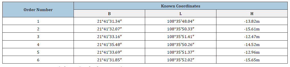
Table 3:Measurement information for feature points.

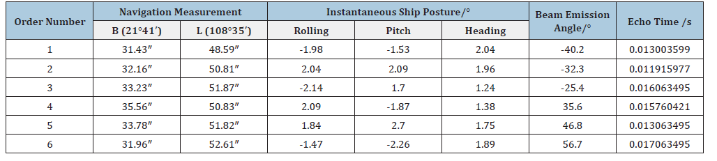
Based on the beam emission angle and echo time data in the table above, observation point was obtained by performing constant-gradient sound line tracking using the measured sound velocity profile from field surveys. Taking the calibration measurement points specified in Table 1 as the origin of the local horizontal coordinate system, relevant formulas were applied to convert coordinates expressed in geodetic latitude and longitude into Gaussian coordinates [15] and coordinate deviations were calculated in conjunction with ship attitude data to yield point .

Based on the obtained information, perform calculations using equations (29) to (33)

Let α，β γ denote the yaw deviation angle, pitch deviation angle and roll deviation angle respectively. According to the coordinate system transformation rules [16], can be expressed as follows:

By decomposing using mathematics, α =2.36 , β =-3.07 , γ =1.54 . Compared with the “actual values” in Table 1, the deviations are Δα= 0.01°, Δβ = 0.02° and Δγ = 0.01°. This demonstrates that the proposed algorithm effectively determines the angle installation deviation of the transducer. Due to practical constraints, this experiment utilized seabed topography obtained after traditional installation deviation calibration and various routine corrections as the reference datum, while using uncalibrated seabed data for actual measurements. Installation deviations were comprehensively calibrated by leveraging topographic feature points. The results demonstrate that the proposed comprehensive calibration method based on total least squares can effectively determine deviation values. Theoretically, this algorithm exhibits superior accuracy compared to traditional separate calibration methods and other comprehensive calibration approaches based on general least squares principles, though further experimental analysis and validation are required.

Calibration of transducer installation deviations is a critical preparatory step before formal multi-beam bathymetry operations commence, directly impacting data accuracy and final measurement quality. Traditional individual calibration methods often face precision limitations due to their inability to fundamentally address the interdependence among various deviation factors. In contrast, integrated calibration combines multiple deviation parameters into a unified model for simultaneous estimation, overcoming the shortcomings of separate calibration methods and representing the prevailing approach for future transducer installation deviation calibration. Based on current research advancements in integrated calibration worldwide, this paper proposes an algorithm for transducer installation deviation calibration employing total least squares methodology. This algorithm simultaneously accounts for water depth measurement errors, navigation positioning inaccuracies and vessel attitude measurement uncertainties, constructing a comprehensive model within the total least squares framework for rigorous computation. Case studies demonstrate its effective capability in determining transducer installation deviations. However, due to experimental constraints, the superiority of this algorithm over traditional separate calibration and conventional least squares-based integrated calibration has not yet been validated through field measurements-a key focus area for future research by the authors.

1. Zhao Jianhu, Liu Jingnan (2008) Multibeam sounding and image data processing. Wuhan University Press, Wuhan, China.
2. Zhang Zhiwei, Bao Jingyang, Liu Sheng (2017) Plane fitting method for correcting lateral installation deviations of multibeam transducers. Marine Bulletin 36(4): 394-398.
3. Sun Wenchuan, Bao Jingyang, Jin Shaohua, Xiao Fumin, Zhang Zhiwei (2016) A quadratic calibration method for lateral tilt angle deviations of multibeam transducers. Journal of Wuhan University 41(11): 1440-1444.
4. Liu Guoqing, Jin Shaohua, You Baoping, Zhu Muhua (2018) Iterative algorithm for lateral tilt deviation accounting for acoustic line bending. Marine Surveying and Mapping 38(4): 39-42.
5. Huang Xianyuan (2011) Research on data quality control methods for multibeam sounding. PLA University of Information Engineering, Zhengzhou, China.
6. Nicolas Seube (2011) Multibeam sonar performance analysis: Value and application of statistical techniques. International Hydrographic Review, pp. 52-65.
7. Zeng Zhaofu (2018) Research on spatial plane fitting using total least squares methods based on the Partial EIV model. Beijing Surveying and Mapping 32(06): 697-700.
8. Xiong Luyun (2018) Methodology and application research on systematic error treatment in partial EIV models. Donghua University of Technology, China.
9. Guo Jinyun, Xu Xiaofei, Shen Yi (2016) Review of overall least squares algorithms and their measurement applications. Journal of Shandong University of Science and Technology 35(4): 1-12.
10. Liu Jingnan, Zeng Wenxian, Xu Peiliang (2013) Research progress in overall least squares estimation. Journal of Wuhan University 38(5): 505-512.
11. Liu Xianxin, Wang Leyang, Xu Guangyu (2014) Comparison of methods for solving overall least squares adjustment problems. Engineering Surveying 42(7): 40-43.
12. Yu Hang (2016) Joint overall least squares adjustment method and its application research. Donghua University of Technology, China.
13. Luo Jiahong (2000) Introduction to matrix analysis. South China University of Technology Press, Guangzhou, China.
14. Lu Tieding (2010) Theory of overall least squares adjustment and its application in geospatial data processing. Wuhan University, China.
15. Yang Shaohai, Zhang Yanchang (2011) Research on three-dimensional coordinate calculation methods for seabed points in multi-beam measurements. Meteorological, Hydrological and Oceanographic Instruments 2: 1-3.
16. Huang Motao, Zhai Guojun, Xie Xijun (2000) Study on position adjustment and carrier attitude effects in multi-beam and airborne laser depth measurement. Journal of Surveying and Mapping 29(1): 82-88.