Visibility-Based Reconstruction of Light Extinction Coefficient and Its Meteorological Dependence over Agra, India

This study examined the relationships between atmospheric visibility and key meteorological parameters, including Atmospheric Temperature, Relative Humidity (RH), Wind Speed, Wind Direction, and PM2.5 concentrations across three time periods: morning, afternoon, and evening. Pearson and Spearman correlation analyses provided important insights into visibility dynamics. A strong negative correlation was consistently observed between visibility and relative humidity, particularly when RH exceeded 70%, resulting in significantly reduced visibility levels. Similarly, visibility showed a strong negative relationship with PM_2.5 concentrations, confirming the detrimental impact of particulate matter on atmospheric clarity. In contrast, atmospheric temperature exhibited a generally positive correlation with visibility, indicating improved conditions with rising temperatures. The association between visibility and wind speed was more complex; however, higher wind speeds often promoted aerosol dispersion, contributing to better visibility. Additionally, analysis of wind direction categorized into cardinal points revealed notable differences in average visibility depending on air mass origin, suggesting regional influences on atmospheric conditions. Visibility showed a strong negative relationship with PM₂.₅ concentrations, confirming the detrimental impact of particulate matter on atmospheric clarity. Elevated PM₂.₅ levels not only reduce visibility but also contribute significantly to environmental degradation, atmospheric pollution, radiative imbalance, and adverse human health effects. These findings highlight the importance of continuous air quality monitoring and effective pollution mitigation strategies to minimize environmental and public health risks associated with fine particulate matter. Overall, the results identify relative humidity, PM2.5 concentrations, and temperature as primary drivers of visibility variability, with wind dynamics playing a secondary but important role throughout the day. .

Keywords:Visibility; Relative humidity; PM₂.₅; Light extinction coefficient

Air pollution is one of the most urgent environmental challenges of the twenty‑first century, with fine particulate matter (PM_2.5) recognized as a particularly harmful pollutant. PM_2.5 particles, with diameters less than 2.5 micrometers, originate from combustion processes, industrial activity, biomass burning, and natural sources such as dust storms. Their small size allows them to penetrate deep into the respiratory system, causing cardiovascular and respiratory diseases, while also reducing atmospheric visibility through light scattering and absorption. The Global Burden of Disease Study (2023) estimated millions of premature deaths annually attributable to PM_2.5 exposure, reinforcing the pollutant’s dual role as a health hazard and an environmental stressor [1].

Beyond health impacts, PM_2.5 is a major contributor to haze and visibility reduction. Hao, Wang, and Wu reconstructed long‑term PM_2.5 concentrations using visibility observations across the Northern Hemisphere, demonstrating that visibility data can serve as a reliable proxy for particulate pollution [2]. Yin emphasized the importance of integrating meteorological parameters such as humidity and temperature into visibility models, noting that high humidity enhances particle growth and scattering efficiency [3]. These findings highlight the global relevance of visibility studies in understanding particulate pollution.

Recognizing the severity of PM_2.5 pollution, the World Health Organization (WHO) issued its Global Air Quality Guidelines, recommending an annual mean concentration of 5μg/m³ and a 24‑hour mean of 15μg/m³ [4]. The WHO Air Quality Database further revealed that most urban centers worldwide exceed these thresholds, with South Asia among the most affected regions [5]. Complementing this, the IQ Air World Air Quality Report ranked India among the countries with the highest PM_2.5 exposure, underscoring the urgency of stricter standards [6].

India’s Central Pollution Control Board (CPCB) has set National Ambient Air Quality Standards (NAAQS) for PM_2.5 at 40μg/m³ annually and 60μg/m³ for 24 hours. These thresholds are far less stringent than WHO’s guidelines, reflecting the challenges of balancing public health with economic growth. CPCB’s Annual Report 2022- 23 revealed that more than 60% of districts exceeded the national standard, with northern India recording the highest concentrations [7]. Seasonal peaks in winter, driven by stubble burning, traffic, and industrial emissions, exacerbate visibility reduction. The Centre for Science and Environment reported that annual PM2.5 levels rose despite reduced stubble burning, highlighting the role of urban emissions and meteorology [8].

Recent research has deepened understanding of PM_2.5 dynamics in India. Gil‑Alana et al. [9] analyzed persistence and trends in five Indian cities, confirming long‑term deterioration in air quality [10]. Govande et al. [11] applied recurrent neural networks to predict PM_2.5 levels in metropolitan cities, demonstrating the potential of machine learning for early warning systems [9]. Science Advances developed open‑source daily PM_2.5 datasets at 10‑km resolution for India, revealing inequalities in exposure across regions. These studies underscore the need for localized modeling that accounts for both emission sources and meteorological influences [11].

Agra, home to the Taj Mahal, presents a unique case study. Tourism is central to Agra’s economy, and visibility degradation caused by PM_2.5 pollution directly affects the city’s cultural and economic vitality. CPCB monitoring stations consistently show that PM_2.5 concentrations in Agra exceed both national and WHO standards, with winter months recording the highest levels. High humidity enhances particle growth, increasing haze, while temperature inversions trap pollutants near the surface. Poor visibility diminishes visitor experience and affects photography, a key aspect of tourism. Local emission sources include vehicular traffic, brick kilns, biomass burning, and construction dust, creating a complex pollution profile that requires site‑specific modelling.

Despite extensive global research, localized studies in Agra remain limited. Existing models often rely on generalized coefficients that do not capture Agra’s unique atmospheric dynamics. There is a need for empirical extinction equations calibrated with local data, integrating PM_2.5 concentrations and meteorological parameters. This study therefore aims to quantify the relationship between PM_2.5 and visibility in Agra using extinction equations and regression analysis. By comparing local findings with CPCB data and WHO guidelines, the research seeks to provide actionable insights for air quality management and heritage preservation.

Data Collection and Sampling

Site description

Sanjay Place, located in the Civil Lines area of Agra, Uttar Pradesh, is a densely built commercial hub that serves as the focal site for this study. Geographically, it lies at approximately 27.2006°N latitude and 78.0056°E longitude, with an elevation of around 171 meters above sea level. The area is bounded by major arterial roads such as Mahatma Gandhi Road (M.G. Road) to the west and Bhagwan Talkies Crossing to the north, making it one of the busiest traffic zones in the city. The land use is predominantly commercial, comprising banks, government offices, shopping complexes, and eateries, while adjacent residential colonies like Civil Lines and Nehru Nagar contribute additional domestic emissions. The built environment features high-rise buildings, narrow lanes, and limited green cover, creating a street canyon effect that traps pollutants and restricts natural dispersion.

Temporal data collection strategy

Air pollution levels, especially PM2.5, are not constant throughout the day. They change with traffic activity, meteorological conditions, and human behaviour. By measuring in the morning, afternoon, and evening, I have captured these natural fluctuations:

A. Morning (09:00-10:00hrs): Traffic congestion is at its peak, humidity is higher, and temperature inversions often trap pollutants near the ground. This makes morning readings important for understanding worst-case visibility conditions.
B. Afternoon (12:00-13:00hrs): Strong sunlight and atmospheric mixing disperse pollutants. Afternoon readings usually show lower PM2.5 concentrations and better visibility, providing a contrast to morning and evening peaks.
C. Evening (15:00-16:00hrs): Traffic builds up again, temperatures drop, and haze formation becomes more likely. Evening data helps capture the second pollution peak of the day.

Data collection tools

To ensure accurate measurement of particulate matter and visibility, a combination of instrumental and visual methods was employed at the study site. The Low Volume Sampler (LVS) was used for monitoring PM_2.5 concentrations. This instrument operates by drawing ambient air at a controlled flow rate through a filter medium, selectively capturing particles with an aerodynamic diameter of less than 2.5 micrometer. The sampling was done at the top of the building. Sampling was conducted three times daily (morning, afternoon, evening) to capture diurnal variations. Meteorological data is gathered from Central Pollution Control Board (CPCB) regional office and CPCB site [12].

For visibility assessment, a digital camera was employed to record photographic evidence of landmark structures at varying distances from the sampling points. Images were taken at consistent intervals (morning, afternoon, evening) and from fixed vantage points to ensure comparability. The photographs provided qualitative documentation of haze intensity and were later cross‑referenced with PM_2.5 concentrations to establish correlations between particulate load and visibility reduction. Care was taken to maintain uniform camera settings, including focal length and orientation, across all sessions.

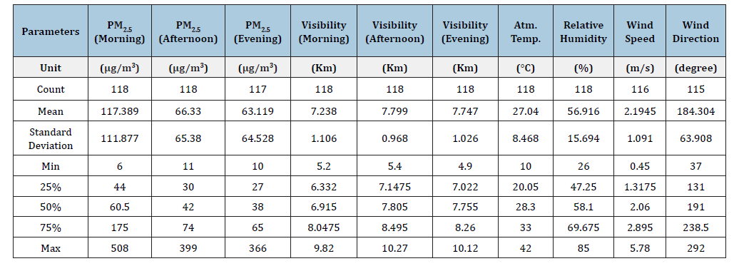
(Table 1)

Table 1:Statistical data of concentration of PM_2.5, Visibility and Meteorological Parameters.

Analysis of Koschmieder’s law for visibility to extinction coefficient conversion

Visual Range (VR) is a widely used indicator of atmospheric visibility, defined as the maximum distance at which a target can be distinguished against the horizon [13]. The Koschmieder equation is a foundational model in atmospheric science used to quantify visibility. Developed by Hermann Koschmieder in 1924, it is based on the principle that the ability to see a distant object depends on the contrast between that object and the background sky. As light travels through the atmosphere, it is scattered and absorbed by gases and aerosols, which reduces this contrast. Visibility is defined as the farthest distance at which a dark object can be distinguished against the horizon sky when the contrast between the object and background falls to a threshold value of approximately 2%.

Mathematically, the Koschmieder equation is expressed as:

Data acquisition and quality assurance

A multi-source data acquisition strategy combined remote sensing, GPS field surveys, structured household questionnaires, and archival review (Table 1). This triangulation mitigates the documented limitations of single data streams in data-scarce Sub- Saharan African environments [9,11].

Rigorous quality assurance comprised: (a) spatial accuracy verification by cross-referencing GPS points against satellite imagery (>5m offset flagged for re-verification; RMSE calculated); (b) topological integrity checks using ArcGIS topology rules to detect and correct dangling nodes, undershoots, and disconnected segments; and (c) attribute completeness audits validating one-toone correspondence of unique household identifiers across Access and ArcGIS, with mismatch rates documented and resolved.

Spatial database construction and ODBC integration

The spatial database was constructed in ArcGIS (version 10.x) as a geodatabase comprising household point locations, classified road network polylines, administrative boundary polygons, and collection infrastructure, all standardized to WGS 84/UTM Zone 32N. The critical innovation is the dynamic ODBC linkage between the ArcGIS geodatabase and a relational Microsoft Access database, enabling bidirectional real-time synchronization. The Access schema was structured around a primary key (unique household ID) linking demographics, subscription details, and agent assignments, with referential integrity constraints enforced. Synchronization was validated through controlled test updates confirming field-level consistency across platforms. The modular schema is compatible with QGIS, PostGIS, and PostgreSQL, reducing vendor lock-in.

Network analysis and route optimization

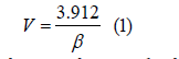
Where, V represents the visual range (in km) and σ denotes the atmospheric extinction coefficient (in km^-1). The extinction coefficient accounts for both scattering and absorption processes in the atmosphere. In practice, σ can be estimated using particulate matter concentrations, especially fine particles such as PM2.5, along with meteorological parameters like relative humidity. Under humid conditions, PM_2.5 particles absorb water and grow in size, which increases their scattering efficiency and raises the extinction coefficient, thereby reducing visibility [14].

This equation provides a direct link between air pollution levels and visual range, making it a widely applied tool in studies of air quality, haze formation, and environmental monitoring.

β_Rayleigh: Scattering by air molecules (important in clean air).
β _Aerosol: Scattering and absorption by particles such as PM_2.5, dust, smoke.
β_Gas: Absorption by gases like ozone, nitrogen dioxide, or water vapour.

β is the extinction coefficient that quantifies how much light is scattered and absorbed in the atmosphere. It is the bridge between air pollution (PM_2.5, gases) and visibility, and the Koschmieder equation uses it to calculate visual range [15].

Nevertheless, Koschmieder’s law remains the most practical first-order method for estimating visibility because it requires only a single key parameter: the extinction coefficient. This has led to its continued adoption in modern air-quality applications, including empirical models linking particulate matter (PM₂.₅) concentrations to degradation in visibility. It therefore maintains both scientific and operational importance in atmospheric optics and environmental monitoring.

The Spearman rank correlation coefficient is a non‑parametric statistic designed to measure the strength and direction of association between two variables based on their ranked values. Unlike Pearson’s correlation, which assumes linearity and normally distributed data, Spearman’s method evaluates monotonic relationships and is therefore more robust when data are skewed, ordinal, or influenced by outliers. This makes it particularly useful in environmental and health sciences, where variables such as humidity, particulate matter, or visibility often interact in non‑linear ways. Researchers have emphasized its versatility across disciplines, noting that it can reliably capture associations even when traditional parametric assumptions are violated [16,17]. More recent applications highlight its effectiveness in analyzing meteorological datasets, biomedical outcomes, and social science variables, reinforcing its role as a flexible tool for correlation analysis in complex real‑world contexts [18-20].

Formula for Spearman Correlation

For paired observations, the Spearman correlation coefficient (ρ) is calculated as:

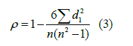
Where: d_i=difference between the ranks of each pair of observations, n=number of observations. If there are tied ranks, average ranks are assigned, and the formula can also be computed using the Pearson correlation applied to ranked data.

Pearson’s correlation coefficient has been widely adopted in environmental research to explore linear associations between air quality indicators and visibility. In studies conducted in Delhi, researchers reported that increases in fine particulate matter were consistently linked with reductions in visual range, highlighting a strong negative correlation between aerosol concentrations and atmospheric clarity [21]. Similar findings were observed in Hong Kong, where meteorological stagnation combined with elevated particulate levels produced significant linear relationships with degraded visibility [22]. Work in China further demonstrated that secondary aerosols such as sulphates and nitrates were closely correlated with visibility loss, reinforcing the role of chemical composition in shaping optical properties of the atmosphere [23]. At Incheon International Airport in South Korea, Pearson correlation analysis revealed that PM2.5 was the most influential factor in reducing visibility, particularly under humid conditions that enhanced light scattering [24]. Collectively, these studies illustrate the effectiveness of Pearson correlation in quantifying pollutant-visibility relationships across diverse geographic regions, providing a methodological foundation for similar analyses in Agra.

Formula for Pearson Correlation: For n paired observations (x_i, y_i), the Pearson correlation coefficient r is calculated as:

Where: x_i, y_i = individual data points, = means of the variables and r ranges between -1 and +1 [24].

Qualitative analysis

To quantify atmospheric visibility, the raw sampling photographs were transformed into visual range values using dedicated image-processing software. The software computes visibility by evaluating scene contrast degradation relative to known targets or background luminance profiles. This approach aligns with previous studies where digital photographs have been successfully used to estimate visibility and haze intensity through contrast-based algorithms [25-27]. Furthermore, such methods complement theoretical formulations such as Koschmieder’s law, where visibility is inversely proportional to the atmospheric extinction coefficient [14].

Effect PM_2.5 on visibility

Figure 1:Diurnal comparative scatter plot between PM2.5 and Visibility.

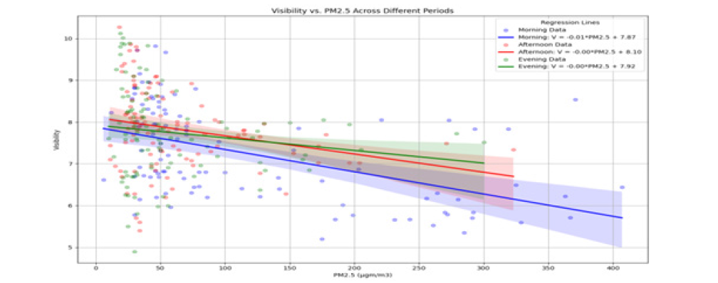
Figure 1 shows the relationship between PM₂.₅ concentration and visibility exhibits clear diurnal variability. During the morning hours, a pronounced inverse association is observed, with visibility decreasing as PM₂.₅ concentrations increase, as indicated by the distinct downward trend in the scatter plot and supported by moderate negative Pearson (r=-0.461) and Spearman (ρ= -0.527) correlation coefficients. The slightly stronger Spearman correlation suggests that the association is consistently negative but not strictly linear, likely influenced by stable atmospheric conditions and a shallow boundary layer that enhance particle accumulation and light extinction. In contrast, the afternoon period shows a substantially weaker relationship, with a scattered distribution of data points and a marginally negative regression slope, reflected in low Pearson (r= -0.139) and Spearman (ρ= -0.273) correlations. This weakening indicates increased atmospheric mixing and dispersion during daytime, which reduces the direct influence of PM₂.₅ on visibility. The evening period exhibits the weakest association among all three-time intervals, characterized by highly dispersed data and very low negative correlations (Pearson r= -0.115; Spearman ρ= -0.220), suggesting that PM₂.₅ has minimal control over visibility during this time. Overall, the results demonstrate that PM₂.₅ exerts the greatest impact on visibility during morning hours, with its influence progressively diminishing in the afternoon and evening, emphasizing the role of diurnal meteorological and boundary layer processes in modulating particulate matter-visibility relationships [28].

Figure 2 shows the diurnal variation of visibility reveals a clear and consistent temporal pattern across the observation period. Afternoon visibility is generally higher and more stable than both morning and evening visibility, indicating comparatively clearer atmospheric conditions during afternoon hours. This enhanced visibility is likely associated with increased solar heating, which promotes stronger vertical mixing and dispersion of aerosols, thereby reducing light extinction. In contrast, morning visibility exhibits greater variability and is frequently lower than afternoon values, with several instances of pronounced reductions. These morning dips may be attributed to stable atmospheric conditions, shallow boundary layer heights, and the accumulation of pollutants during overnight hours. Evening visibility also shows noticeable fluctuations and is typically lower than afternoon visibility, often following trends similar to the morning period but remaining consistently below afternoon levels. The time-series analysis further highlights distinct day-to-day variability, where simultaneous rises or drops in visibility across all three periods suggest the influence of broader synoptic or regional atmospheric conditions. Conversely, days on which one time period deviates markedly from the others indicate the role of local or time-specific processes. Overall, the observed diurnal pattern underscores the dominant influence of atmospheric mixing, boundary layer dynamics, and pollutant accumulation on visibility throughout the day.

Figure 2:Dynamics of atmospheric visibility from august 2021 to July 2022.

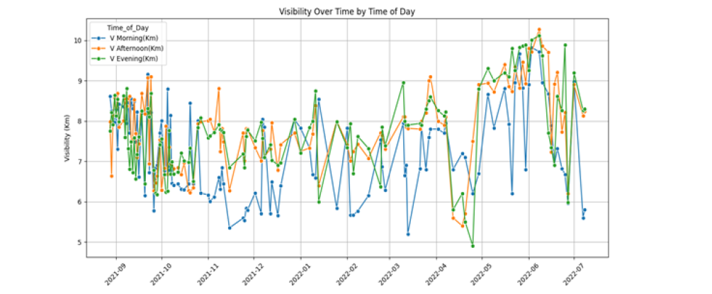
Diurnal variation of visibility

Figure 2 shows the diurnal variation of visibility reveals a clear and consistent temporal pattern across the observation period. Afternoon visibility is generally higher and more stable than both morning and evening visibility, indicating comparatively clearer atmospheric conditions during afternoon hours. This enhanced visibility is likely associated with increased solar heating, which promotes stronger vertical mixing and dispersion of aerosols, thereby reducing light extinction. In contrast, morning visibility exhibits greater variability and is frequently lower than afternoon values, with several instances of pronounced reductions. These morning dips may be attributed to stable atmospheric conditions, shallow boundary layer heights, and the accumulation of pollutants during overnight hours. Evening visibility also shows noticeable fluctuations and is typically lower than afternoon visibility, often following trends similar to the morning period but remaining consistently below afternoon levels. The time-series analysis further highlights distinct day-to-day variability, where simultaneous rises or drops in visibility across all three periods suggest the influence of broader synoptic or regional atmospheric conditions. Conversely, days on which one time period deviates markedly from the others indicate the role of local or time-specific processes. Overall, the observed diurnal pattern underscores the dominant influence of atmospheric mixing, boundary layer dynamics, and pollutant accumulation on visibility throughout the day.

Effect of meteorological parameters on visibility

Effect of atmospheric temperature: Figure 3 shows the relationship between atmospheric temperature and visibility across different times of the day reveals a weak but consistent pattern. Atmospheric temperature during the study period ranges approximately from 10 °C to 42 °C, with most observations clustered around a mean value of 27.11 °C. Visibility across all time periods generally lies between 5km and 10km, with morning visibility ranging from 5.2km to 9.82km, afternoon visibility from 5.4km to 10.27km, and evening visibility from 4.9 km to 10.12km. The regression analysis indicates a very slight negative relationship between temperature and visibility for all three periods. In the morning, the regression line shows a marginal downward slope, suggesting that an increase in atmospheric temperature is associated with a minor reduction in visibility, with an average morning visibility of approximately 7.24km. A similar weak negative trend is observed in the afternoon, where visibility is generally higher than in the morning, averaging about 7.84km, but still exhibits a small decline with increasing temperature. The evening period follows the same pattern, with an average visibility of around 7.77km and a slight negative slope in the regression line. Overall, these results indicate that atmospheric temperature alone exerts only a limited influence on visibility, and that other factors such as aerosol loading, humidity, and atmospheric stability likely play a more dominant role in controlling visibility variations.

Figure 3:Comparison of visibility in morning afternoon and evening with atmospheric temperature.

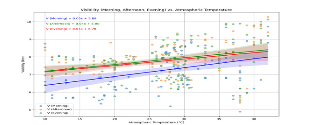
Figure 4:Comparison of visibility in morning afternoon and evening with relative humidity.

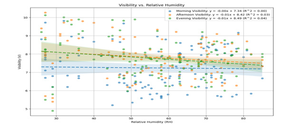
Effect of relative humidity: Figure 4 shows the correlation analysis between visibility and relative humidity reveals a consistently weak inverse relationship across all diurnal periods. In the morning, the Pearson correlation coefficient is -0.03 with an R² value of 0.00, indicating a negligible negative relationship and virtually no explanatory power of relative humidity on morning visibility. During the afternoon, the negative association becomes slightly stronger (r= -0.18; R²=0.03), suggesting that increases in relative humidity are accompanied by minor reductions in visibility, although relative humidity explains only 3% of the observed variability. The evening period exhibits the strongest, yet still weak, negative relationship (r= -0.20; R²=0.04), indicating that relative humidity accounts for approximately 4% of the variance in evening visibility. This comparatively stronger evening influence may be linked to cooling temperatures, increased atmospheric stability, and a greater likelihood of moisture-driven haze or mist formation. Overall, despite the well-known physical mechanisms through which relative humidity can reduce visibility via aerosol hygroscopic growth and enhanced light scattering, the low correlation and R² values in this dataset indicate that relative humidity alone has limited predictive capability. These findings suggest that visibility is governed by a combination of interacting factors, including aerosol loading, meteorological conditions, and atmospheric dynamics, rather than by relative humidity in isolation.

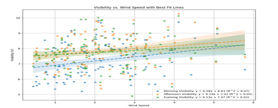
Effect of wind speed: Figure 5 shows the correlation analysis indicates that wind speed has only a weak influence on visibility across all time periods. In the morning, the Pearson correlation coefficient (r=0.27) and the corresponding R² value of 0.07 suggest a very weak positive linear relationship, with wind speed accounting for only 7% of the variability in morning visibility. Similarly, during the afternoon, a weak positive association is observed (r=0.22; R²=0.05), indicating that wind speed explains merely 5% of the variance in visibility. The weakest relationship occurs in the evening, where the Pearson correlation coefficient (r=0.14) and R² value of 0.02 demonstrate an extremely weak positive linear relationship, with wind speed contributing to only 2% of the observed variation in visibility. Overall, although higher wind speeds tend to be associated with marginal improvements in visibility due to enhanced dispersion of pollutants, the low correlation and R² values across all periods indicate that wind speed alone is a poor predictor of visibility. This suggests that other factors, such as aerosol concentration, relative humidity, and atmospheric stability, play a more dominant role in controlling visibility variations.

Figure 5:Comparison of visibility during morning, afternoon, and evening under different wind speeds

Effect of wind direction

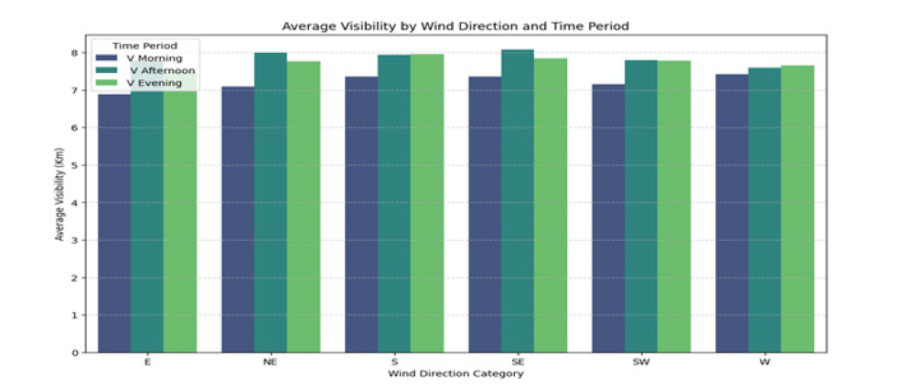
Figure 6 shows the Average Visibility by Wind Direction and Time Period bar plot provides a clear visualization of how wind direction influences visibility under different diurnal conditions. The plot enables the identification of specific wind directions that are consistently associated with higher average visibility, suggesting the transport of relatively clean air masses and enhanced dispersion from those directions. In contrast, wind directions linked to lower average visibility likely represent the advection of polluted air, proximity to emission sources, or meteorological conditions favourable for fog or haze formation. The comparison across morning, afternoon, and evening periods further reveals temporal variability in these wind-visibility relationships, reflecting changes in atmospheric dynamics, boundary layer development, and local emission activity throughout the day. Such diurnal shifts indicate that the influence of wind direction on visibility is not static but evolves with time, emphasizing the importance of air-mass origin and transport pathways in controlling visibility.

Figure 6:Comparison of visibility during morning, afternoon, and evening under different wind speeds.

Correlation matrix of meteorological parameters

Figure 7:Pearson and spearman correlation matrix of visibility with different meteorological parameters.

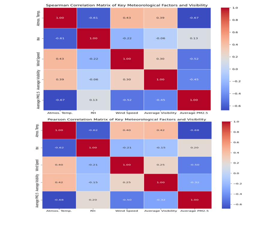
Figure 7 shows the comparative analysis of Pearson and Spearman correlation matrices provides insight into both the linear and monotonic relationships among key meteorological and pollution parameters affecting visibility. Strong agreement between the two-correlation metrics is observed for several pairs, such as atmospheric temperature and relative humidity (Pearson: -0.62, Spearman: -0.61), temperature and average PM₂.₅ (Pearson: -0.68, Spearman: -0.67), and wind speed and average PM₂.₅ (Pearson: -0.50, Spearman: -0.52), indicating that these relationships are robustly both linear and monotonic. Differences between the two measures reveal more nuanced trends. For instance, relative humidity versus average visibility shows a weaker Spearman correlation (-0.06) compared to Pearson (-0.15), suggesting that the rank-order consistency of this relationship is limited and may be influenced by outliers or non-linearities. Conversely, wind speed versus average visibility exhibits a slightly stronger Spearman correlation (0.30) than Pearson (0.25), implying that higher wind speeds consistently correspond to higher visibility ranks, even if the linear relationship is modest. The most notable difference is seen in average visibility versus average PM₂.₅, where the Spearman correlation (-0.45) is substantially stronger than Pearson (-0.32), indicating a reliably inverse monotonic relationship between PM₂.₅ and visibility despite potential non-linear behaviour. Overall, this comparison highlights that while meteorological factors such as RH and wind speed have limited direct influence on visibility, PM₂.₅ exerts a dominant and consistently inverse effect, and that monotonic measures like Spearman correlation are particularly useful for capturing consistent trends that may not be strictly linear.

The analysis demonstrates that visibility is governed by a complex interplay of aerosol loading and meteorological conditions, with clear diurnal variability in the dominant controlling mechanisms. The morning period exhibits the strongest inverse relationship between PM₂.₅ concentration and visibility, indicating that higher particulate pollution levels are more directly associated with reduced visibility during this time. This stronger morning sensitivity is likely driven by overnight pollutant accumulation, elevated relative humidity, all of which enhance aerosol light scattering and extinction. In contrast, the PM₂.₅ and visibility relationship weakens considerably during the afternoon and evening, suggesting that either PM₂.₅ concentrations exert a reduced direct influence or that other atmospheric processes become more dominant. Consistent with this, afternoons generally experience better visibility than mornings and evenings, reflecting enhanced solar heating and improved dispersion of aerosols.

Meteorological factors further modulate visibility across the day. Relative humidity and PM₂.₅ act to reduce visibility by promoting hygroscopic growth of aerosols and increasing light extinction, whereas higher temperatures and wind speeds generally improve visibility by enhancing atmospheric mixing and pollutant dispersion. Wind direction plays a particularly important role by determining the origin of air masses reaching the study area, thereby influencing whether cleaner or more polluted air is adverted. Understanding wind direction is therefore critical for identifying local and regional source influences and explaining dayto- day variability in visibility.

These physical processes are also reflected in the behaviour of the atmospheric extinction coefficient (β). Morning β values range from 0.3984 to 0.7523, indicating substantial variability in light extinction associated with changing pollution and humidity conditions. Afternoon β values are comparatively lower, ranging from 0.3809 to 0.7244, consistent with improved dispersion and higher visibility during this period. The evening shows the widest range, with β varying from 0.3866 to 0.7984, suggesting renewed pollutant accumulation and increased atmospheric stability. Overall, the combined evidence indicates that visibility cannot be attributed to a single controlling factor; rather, it results from the coupled effects of aerosol concentration, hygroscopic growth, and air-mass transport, with their relative importance varying throughout the diurnal cycle.

The authors acknowledge the institutional support provided by the college for facilitating this research work. The author also gratefully acknowledges the Central Pollution Control Board (CPCB) for providing air quality data, the India Meteorological Department (IMD) for meteorological observations, and other publicly available data sources used in this study. This research did not receive any specific grant from funding agencies in the public, commercial, or not-for-profit sectors.

This research did not receive any specific grant from funding agencies in the public, commercial, or not-for-profit sectors..

1. Wenhua Y, Tingting Y, Yiwen Z, Rongbin X, Yadong L, et al. (2023) Global estimates of daily ambient fine particulate matter exposure. Lancet Planet Health 7(3): e209-e218.
2. Hao H, Wang K, Wu G, Liu J, Li J (2024). PM₂.₅ concentrations based on near-surface visibility in the northern hemisphere (1959-2022). Earth Syst Sci Data 16(9): 4051-4076.
3. Yin PY (2025) A review on PM₂.₅ sources, mass prediction, and association analysis. Sustainability 17(3): 1101.
4. World Health Organization (2021) WHO global air quality guidelines. World Health Organization, Geneva, Switzerland.
5. World Health Organization (2022) Air quality database. (5^th edn), World Health Organization, Geneva, Switzerland.
6. IQAir (2023) World Air Quality Report 2023. IQAir, Switzerland.
7. IQAir (2024) World Air Quality Report 2024. IQAir, Switzerland.
8. Central Pollution Control Board (2024) Annual report 2022-23. CPCB, New Delhi, India.
9. Gil-Alana LA, Carmona-González N (2025) Particulate matter 2.5 (PM₅): Persistence and trends in PM₂.₅ in five Indian cities. Atmosphere 16(5): 534.
10. Centre for Science and Environment (2024) End of winter report 2023-24: Spread and scale of air pollution crisis. CSE, New Delhi, India.
11. Govande R (2024) Predicting PM₂.₅ levels in Indian metropolitan cities using recurrent neural networks. Earth Sci Inform.
12. Kawano A, Kelp M, Qiu M, Singh K, Chaturvedi E, et al. (2025) Improved daily PM₂.₅ estimates in India reveal inequalities in recent enhancement of air quality. Sci Adv 11(4): eadq1071.
13. Central Pollution Control Board (2022) Real-time air quality monitoring data.
14. Middleton WEK (1952) Vision through the Atmosphere. University of Toronto Press, Toronto, Canada.
15. Koschmieder H (1924) Theory of horizontal sight distance. Beitr Phys Freien Atmos 12: 171-181.
16. Lee Z, Shang S (2016) Visibility: How applicable is the century-old Koschmieder model? J Atmos Sci 73(1): 31-47.
17. Spearman C (1904) The proof and measurement of association between two things. Am J Psychol 15(1): 72-101.
18. Mukaka MM (2012) A guide to appropriate use of correlation coefficient in medical research. Malawi Med J 24(3): 69-71.
19. Das S (2025) A study on effectiveness of Spearman’s rank correlation coefficient under generalized partially linear regression. Int J Creat Res Thoughts 13(3): 500-510.
20. Kumar P (2021) Significance of Spearman’s rank correlation coefficient. J Stat Appl 18(2): 45-53.
21. Alsaqr AM (2020) Remarks on the use of Pearson’s and Spearman’s correlation coefficients in assessing relationships in ophthalmic data. Afr Vis Eye Health 80(1): 1-6.
22. Singh A, Dey S (2012) Influence of aerosol composition on visibility in megacity Delhi. Atmos Environ 62: 367-373.
23. Cheung YT (2005) Influence of meteorology on visibility in Hong Kong. Atmos Environ 39(31): 5967-5977.
24. Wang Y (2014) Sulfate, nitrate, and ammonium aerosols in relation to visibility in China. Atmos Chem Phys 14: 10233-10245.
25. Won WS, Rosy O, Woojoo L, Ki-Young K, Sungkwan K, et al. (2020) Impact of fine particulate matter on visibility at Incheon International Airport, South Korea. Aerosol Air Qual Res 20(5): 1048-1061.
26. Khedekar S, Thakare S (2023) Correlation analysis of atmospheric pollutants and meteorological factors using statistical tools in Pune, Maharashtra. Int J Environ Sci Technol 20(5): 421-430.
27. Cai Y (2016) Visibility estimation from digital images based on contrast and atmospheric scattering. Atmos Environ 124: 48-59.
28. Baumer D, Versick S, Vogel B (2008) Determination of the visibility using a digital panorama camera. Atmospheric Environment 42(11): 2593-2602.