Spatial Models of Ecological Connectivity Between Seagrass Meadow and Mangrove Forest from Los Petenes Biosphere Reserve, Campeche, Mexico

Ecological connectivity connects biological, physical, and chemical elements among sea and land ecosystems. One way to study is through structural and functional connectivity derived from land use and cover. The structural connectivity refers to metrics and landscape heterogeneity. Functional connectivity denotes how well the landscape allows the fauna movement. We utilized structural and functional connectivity to derive a landscape suitability map, which is an index for healthy vegetation and serves as a food indicator for fish. Landscape suitability was the weighted sum of Submerged Aquatic Vegetation (SAV) biovolume, habitat types, and landscape components from the Integral Index of Connectivity. Ecological parameters and species of the SAV were calculated. Marine and terrestrial cover, landscape uses, and digital terrain models were obtained based on remote sensing. Unsuitable anthropogenic land uses and other terrestrial vegetation as a barrier for fish movements have been considered. This assessment was based on the connection between habitat types like mangroves, seagrass, and macroalgae (SAV) and fish with biological food indicators in the “Los Petenes” Biosphere Reserve (LPBR), Mexico. In the marine zone, grain type was derived by an echosounder, and biovolume was calculated from hydroacoustic variables. Fish tracks were identified in two categories “solitary” or “school fish” in the ecograms collected in field trip transects between 2013-2017. These two categories of behavior were evaluated with habitat types and landscape suitability. Hence this study aimed to evaluate the ecological connectivity between landscape suitability, habitat types, fish, and food indicators for detecting fish movement. We proposed four spatial models. Model 1 shows nodes overlapping interactions between solitary and school fish, based on predictor track density. Model 2 directs probability routes for fish movement between suitable landscapes based on data collection references to all fish tracks. In the third and fourth for ecological connectivity, both fish behaviors were evaluated with food meiofauna, and epiphytes present in the sediment and leaves of the SAV. Sound evidence for a high degree of connectivity in the LPBR indicates that the integral models will support spatial planning for promoting sustainable tourism development and ecosystem conservation.

Keywords:Seagrass; Mangroves; Fish tracks; Food indicators; Nodes and routes; Ecological connectivity; Remote sensing

Ecological connectivity is the connection between biological, physical, and chemical elements among sea and land ecosystems elements in complex ecosystem [1-5]. These interactions favor the free flow of matter and energy involving their proper function [6,7]. In particular, connectivity ensures the genetic exchange of species [8-10], an increase in population abundance and biomass [11,12], as well as the availability of resources for community sustenance [13,14]. Ecosystem health is constantly threatened by natural phenomena and anthropogenic factors that directly or indirectly impact its structure and function [15]. One way to assess ecosystem health is through structural and functional connectivity derived from remote sensing line base monitoring of seagrass and mangrove cover, other wetlands, and land use, which measures the spatial metrics of patches. Patches are discrete areas of vegetation that form larger nodes, which can be grouped due to similarities and proximity to larger nodes called components [16]. In the Gulf of Mexico, evaluating the dynamics between marine habitat patches has allowed us to determine the importance of water flow as an interconnection between terrestrial, coastal, and aquatic ecosystems [1]. Also, Krumme [17] argues the importance of mangroves and tides induced fish processes between the submerged mangrove at high water and the subtidal areas at low water on a short-time scale in Brazil. Andrade et al. [18] observed fish distribution dependent on depth using hydroacoustic sonar near a basin in the Amazon River in Brazil. It has also been described that increasing distance from the mangrove decreases juvenile abundance, biomass, and species composition [12]. Vertical and horizontal movements during day and night have been observed in daily migratory patterns for fish and plankton [19]. Mouillot et al. [20] suggested redundant functionality in landscape composition patterns with daily mobility routines during day and night [21,22]. Therefore, fish species come and go at different times, distances, and speeds between seagrass and mangrove ecosystems, complementing routine cycles for feeding, protection, reproduction, and survival for the next stage of their lives.

Hydroacoustic remote sensing is a useful technique that allows for modelling the spatial distribution of fish [17], SAV and bottom types in water bodies [18,23,24] as well as rocky and coral habitats [23]. Hydroacoustic remote sensing has also been shown to be a good tool for identifying fish movement [17,18]. On the other hand, in landscape processes assessments, satellite imagery is useful for detecting seagrass, mangroves, wetlands and land cover use [25]. Both remote sensing techniques were complemented to obtain better results. Engelhard et al. [26] proposed an integral connectivity network with fish that highlights fauna corridors among mangroves, seagrass, and coral reef patches for better protection in Moreton Bay, Australia. Goicolea and Mateo-Sánchez [13] developed probability models of ecological fluxes of species that interact in landscapes affected by land use change in the Iberian Peninsula. Fernandes et al. [27] argue that the effects of seasonality, depth, landscape connectivity, and abiotic conditions influence organism movements. Hence ecological connectivity is supported by structural and functional connectivity and describes the behavior or response of organisms to spatial isolation and landscape processes [28-30]. These landscape components explained movements of juvenile and adult fish or larval drift [1,26,31]. Therefore, these spatial traits are closely linked to the ontogenetic development of nursery areas located near the coast [14,32]. Peterson et al. [1] proposed the concept of “Connectivity Corridor Conservation” for designing and implementing marine protected areas to preserve migratory species habitats.

This study evaluates the ecological connectivity between landscape and seascape suitability and habitat types like mangroves, SAV and fish with biological food indicators. We consider information with unsuitable anthropogenic land uses, like cultivated and other terrestrial vegetation with altitudes above sea level as a barrier for fish movements. We proposed four spatial models. Model 1 shows nodes overlapping trophic interactions between solitary and fish school, based on predictor track density. Second, we direct the likely routes for fish movement between suitable landscapes based on data collection references with all track fish. In the third and fourth models for ecological connectivity, both fish behaviors were assessed with feeding meiofauna and epiphytes present in the sediment and leaves of the SAV. Epiphytism is a form of life that grows on a plant organism [33]. We hypothesize that areas with suitable habitat types, such as mangroves and seagrass, will exhibit higher levels of ecological connectivity, facilitating trophic interactions and fish movement. Additionally, we expect that unsuitable anthropogenic land uses will act as barriers to fish movements, influencing their spatial distribution and ecological interactions with coastal habitats. The integral models will support spatial planning for promoting sustainable tourism development and ecosystems conservation.

Study area

“Los Petenes” Biosphere Reserve (LPBR) is a natural protected area with a total extension of 2,828.57km², located between 90º 49’49.08” W, 19º 51’42.12” N and 90º 27’6.48” W, 20º 38’8.16” N (Figure 1). The LPBR has extensive areas of well-conserved and interconnected terrestrial and marine vegetation cover. The marine zone has an extension of 1,817.64km² and the flooded terrestrial zone with mangroves is 1,011km². Eighty percent of the marine zone is covered by seagrass species Thalassia testudinum (Tt), Syringodium filiforme (Sf), and Halodule wrightii (Hw), which grow monospecifically or mixed with macroalgae, such as Caulerpa paspaloides van wudermannii [34,35], Avrainvillea, Penicillus, Halimeda, and Udotea genera [36]. The terrestrial zone shows preserved and disturbed mangroves of Rhizophora mangle and Laguncularia racemosa, among other riparian wetlands, terrestrial vegetation, water bodies, anthropic development and agricultural and livestock areas [37]. LPBR is a platform of marine sedimentary strata of carbonate rocks (CaCO₃) with almost absent slope not exceeding 10 meters in altitude. The water table is shallow [38], surfacing as water springs due to karstic origin of the Yucatan Peninsula [37]. The Yucatan Peninsula is a relevant biogeographic area nationally, along with the “Ría Celestún” Biosphere Reserve and “El Palmar” State Reserve, forming a unique ecoregion with similar climate and soil characteristics, allowing a connection of unique processes and biodiversity in Mexico [37,39]. This ecoregion was declared wetland of national and international importance on February 2, 2005 (https://www.ramsar.org/).

Figure 1:Location of “Los Petenes” Biosphere Reserve in Campeche, México. (A) Perpendicular and parallel transects to the coast conducted between 2013 and 2017. (B) Solitary and fish school tracks recorded on the transects, bathymetry and Digital terrain Model. (C) Grid of points with fish presence and absence reconstructed using geospatial sources, grain types and epiphytes index

Hydroacoustic remote sensing

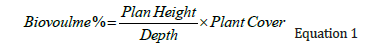
Field collection: The characterization of SAV in the LPBR was performed using a single transducer hydroacoustic echosounder (Biosonics DT-X) with GPS. Approximately 1,211 linear kilometres were covered during dry (March and April), rainy (August and September) and winter (locally known as the “nortes”) (December and February) seasons over seven years of sampling from 2013 to 2023, covering a surface of 1,514km2 [40,41]. In total, 27 perpendicular transects were conducted, reaching up to 24km from the coast, and 6 parallel transects to the coast up to 70 linear km separated by 2 to 3 kilometres, with a navigating speed of 5km/h [42] (Figure 1A). Single Echo Detection Tracks (SEDtracks) were located with their XYZ positions (Figure 1B). A database complemented with fish presence and absence was developed from echosound and other geodatabases (Figure 1C). Vertical information was recorded through pulses that bounce off any “target” (Echo E1: first phase) and receive sound return signals (echoes: E1’ and E2’) at a speed of 1,540m/s with a pulse length of 0.4m per second at a frequency of 430kHz with a 6.4° aperture [43- 45]. Echograms were obtained with graphical representation of the marine profile, recording hydroacoustic variables such as coverage percentage, plant height, and depth. The resulting biovolume is the percentage of aerial biomass of the SAV, obtained from the equation [46] (Figure 2A):

SEDtracks, henceforth referred to as tracks, are small detection fragments of moving fish or fishes, which can be detected individually (samples with one track) or in a school (samples with three or more tracks). Some variables were obtained from each fish track, such as the track density that is the proportion of targets in a swept volume of water (tracks/1000m³) and the average movement speed (m/s) of the fish in the transects [47] (Figure 2B). Simultaneously, the Fractal Dimension (FD) was recorded from three sediment grain types (E2 and E2’), considering roughness and hardness at 20cm from the bottom [43,48-50]. FD values range from 0 to 3, corresponding to fine, medium and coarse sand. Grain type is classified according to traits, from soft and simple grains to harder and complex grain [45,51]. Echograms were analyzed using Visual Aquatic 1.0 post-processing software [52] (Figure 2C).

Figure 2:(A) Field data collection method using the echosounder and recorded hydroacoustic variables. (B) Collection of solitary and fish school tracks from the vessel. (C) Echogram showing coverage and plant height information, depth, sediment grain type, and fish tracks marked in the water column.

A. Meiofauna index: A layer containing sediment grain types from field samples with the echosounder using ordinary kriging interpolation was employed [53]. The sediment grain type variable was used as an indicator of food availability for solitary fish, being significant and correlated with track density for solitary fish in the LPBR. With spatial tools, we created 250 random points, 150 were selected within coarse sand and hard sediment grain types. Based on published dietary references, the hypothesis is that solitary fish, mainly carnivorous, could also be planktivorous or detritivores, and omnivorous habits prefer coarse and hard bottoms rather than medium and soft bottom to feeding [54]. For this reason, a greater number of points were selected for course and hard sediments.
B. Epiphyte index: A layer containing seagrass heights measured in the field with the echosounder and processed using ordinary kriging interpolation was utilized [41,55]. A total of 250 random points were selected from heights. The tallest correspond to S. filiforme that were considered more important as an indicator of food availability, showing highest epiphytic biomass in the LPBR [56,40]. Heights ranging between 16 and 54cm had the greatest weight for school fish. For the medium height (16 to 31cm) and small size (<15cm) ranges, 100 and 50 points were selected, respectively. Additionally, data from 13 collection stations with mean shoot values per square meter of the T. testudinum species were used [40]. Points with shoot measurements >1500 shoots/m² were considered more important for direct routes, while those with less than 500 shoots/m² were deemed less significant for school fish.
C. Track density: A layer containing track density from fish tracks samples with the echosounder was created and employed to interpolate data points using ordinary kriging following the same methods as epiphytes and meiofauna index, described in the previous sections. Model 1 represents nodes with trophic interaction between solitary and school fish based on interpolated track density layer. Overlap nodes were defined at <3000m minimum distance between them. These fish nodes only occur in the marine area of the LPBR since it includes only field samples with the echosounder

Ecological parameters of SAV: Alongside the transects with echosounder, video-transects were recorded using an underwater camera (Sea Viewer). Over the sampling years, 374,998-point occurrences with geographical coordinates were obtained. Additionally, 143 in situ underwater verifications were conducted to confirm the presence of SAV. The in situ record of SAV species was used to calculate basic ecological parameters such as relative dominance, density, and relative frequency of aquatic plants. From these estimates, the Shannon Diversity Index, species evenness, and the Importance Value Index (IVI) of the SAV were calculated and used as input data to create a landscape suitability map using hierarchical decision analysis together with the hydroacoustic variable biovolume. It is important to note that the fish species were not identified in areas where tracks were located using the echosounder. Basic ecological parameters associated with fish were not calculated; only solitary tracks were differentiated from fish school tracks visible in the echograms. Additionally, to exemplify ecological connectivity we assume a trophic interaction between solitary fish as carnivorous and school fish as an herbivorous based on the food preferences recorded in references from LPBR for each social organization [57-59].

Satellite remote sensing

Structural connectivity: The National Commission for the Knowledge and Use of Biodiversity of Mexico (CONABIO) developed a Mangrove Monitoring System to detect land cover, land use, and vegetation on the Mexican coasts. This program was useful for deriving the Integral Index of Connectivity (IIC) in the LPBR. The study of landscape metrics allowed for recognizing the landscapes with the highest number of patches, nodes, and components [60]. ‘Patches’ represent discrete areas whose nature varies depending on the object of study [29]; from these patches, larger ‘nodes’ are formed, made up of two or more patches of coverage. These nodes are grouped into clusters termed landscape components [16]. Landscape heterogeneity was identified through metrics including the number of landscape patches or nodes with higher connectivity, average patch area, patch density, average patch size, patch shape index, and patch complexity using the Patch Analyst plugin in ArcGIS 10.6 [61]. The IIC obtained from components using the CONEFOR Senoseoide 2.6 software proposed by Saura and Pascual- Hortal [30].

Landscape suitability map: Landscape metrics and structural connectivity within LPBR were calculated using hydroacoustic remote sensing cartography complemented with satellite information available in the Geoportal1 of CONABIO. For the terrestrial area of the LPBR, land use and vegetation maps associated with coastal zones adjacent to mangroves in Mexico 2015 were derived from Sentinel 2A [62], as well as IIC [63] and the DTM were utilized to define barriers to fish movement towards internal mangrove areas and caves where they have the possibility to cross between ecosystems [64]. Regarding the marine zone, layers of relative dominance, frequency, density, IVI and SAV biovolume provided by CONABIO´s Geoportal along with landscape components were used [60]. The experimental design encompasses multiple spatial numerical and categorical variables; hence different remote sensing methods were used to determine the ecological connectivity of the wetlands within the LPBR with fish (Figure 3). To estimate landscape suitability, five evaluation criteria were employed, and the mentioned thematic layers were considered as evaluation criteria. A multicriteria hierarchical analysis with minimal inconsistency was conducted using Thomas Saaty’s method [65] in SuperDecisions v 3.12 software2. A scale from one to nine was established, where nine indicates the highest importance and one is equal importance among criteria. Weighted scores for the criteria were obtained through group consensus. Landscape suitability resulted in four categories: 1) Unsuitable, 2) Suitable, 3) Very suitable and 4) The most suitable for fish ecological connectivity within the LPBR. The same method was implemented for habitat type criteria for fish preference.

Figure 3:Remote sensing tools and cartographic inputs used to obtain the landscape suitability map and ecological connectivity of the “Los Petenes” Biosphere Reserve, Campeche.

Statistical analyses

Shapiro-Wilk tests were applied to all variables, considering the null hypothesis of data normality, which was rejected in all cases (p=2.2e-16, α=0.05). The response variable, track density, was square-root transformed to handle multiple values close to zero. The numeric variables and connectivity factors, depth, meiofauna, epiphyte index, landscape suitability, habitat types, patch area and route distances were joined in ArcGIS 10.6., in order to explore the database. Numeric variables were selected based on Pearson correlation. The model design was unbalanced, complex, and heterogeneous as it combines information from diverse sources. An experimental test using permutation-based Analysis of Variance (PERMANOVA) was performed to examine the behavior of the track density variable as a function to the distance to the mangrove, landscape suitability and habitat types [66]. Euclidean distances between each centroid of points with solitary tracks, fish schools and all tracks were permuted 9999 times with the original points [66]. There was sufficient evidence to reject variance homogeneity (p=2.2e-16, α= 0.05) as there are differences among both behaviors and among levels of the evaluated factors. A pairwise test was conducted to reveal which factors were different and their degree of significance in RStudio [67]. GLM with different combinations of predictor variables were used to describe non-linear relationships between variables in RStudio. The resulting models were estimated and subsequently compared via the Akaike Information Criterion (AIC). Deviation, null deviation, mean squared error, and prediction probability were calculated to select the model that best explained data behavior with the least prediction error. The models operated with multiple variables, considering variance heterogeneity and assuming variable independence [68]. Based on the results, variables influencing fish movements were identified. These models aided in weighing nodes and connections of fish in suitable landscapes and habitat types.

Fish routes

An exhaustive literature review was conducted to identify sources providing geographic information on fish presence in areas where fish tracks were not located using the echosounder, such as the Global Biodiversity Information Facility (GBIF)3, the National Biodiversity Information System of Mexico (SNIB)4, the Gulf of Mexico Research Consortium (CIGOM)5, and the National Institute of Statistics and Geography (INEGI)6. Those data points were coded with 1/Presence and 0/absence and analyzed as a binary model. Absences were extracted from the same echosoundercreated transects where no fish were located, supported by random selection tools within subsets in QGIS 2.18.15. Some points were discarded where fish presence was not feasible, such as anthropogenic, agricultural, and livestock land uses, unsuitable for fish movement or with excessive terrain elevation, identified from a Digital Terrain Model (DTM) obtained using LIDAR data [64]. The DTM contained suitable depths of up to -14m, allowing fish to move through existing underground caves in the mangrove-flooded area. Certain areas function as barriers to fish passage, mainly in the central zone of the LPBR. A network of potential movement routes was developed with Euclidean distances from edge to edge using the CONEFOR plug-in ArcGIS 10.6, reaching up to 20,000m from XYZ coordinates at the extreme western boundary of the LPBR to fish XYZ presences at the opposite eastern extreme where there are entrances of water from flooded areas of mangrove. The zones considered to be priority fish destinations with the greatest weight and direction, where the water outputs and entrances known as ‘El Remate,’ ‘La Granja,’ ‘Ixpuc,’ ‘Las Bocas,’ ‘Huayamil,’ ‘Hovonche,’ ‘Peteneyac,’ ‘Jaina,’ ‘Las playitas,’ ‘Ensenada,’ ‘Hampolol’ and ‘Río Verde.’ (Figure 1). The recorded depth ranges within the marine zone vary from -0.5m to -7.03m, which do not represent a barrier to fish movement [41,56]. The water level fluctuation during the rainy season does not exceed -0.5m depth. Pérez-Ceballos et al. [69] show that in these mangrove areas, near Campeche, the maximum registered elevation is 0.28±0.08 meters above sea level. Annually, the hydroperiod oscillates between 0.04 -0.12m.a.s.l. This border strip is called shoreline. Model 2 represents the movement routes indicating fish dispersion among suitability landscapes of the LPBR. A Generalized Linear Model (GLM) was applied to establish a linear component, which was fitted to the response variable, presence and absence with landscape suitability map [70]. Connections covered almost all wetlands in the LPBR. Distances ranged from the geographic positions of tracks to mangrove entrances in a range between 700m to a maximum of 40,000m distance; this range is defined by the critical distance to access resources within the flooded area (Table 1).

Table 1:Nodes and links models proposed for ecological connectivity analysis.

Ecological connectivity

In the Yucatan Peninsula there are numerous ecological and descriptive studies of the dynamics of the most abundant fish species that help us to relate the published information with proposed models [11,71-74]. In the LPBR, the number of fish aggregations per unit area that move within habitat types of preferences have been documented [38,75-78]. These information help to weight habitat types, meiofauna and epiphyte index through group consensus and was related with echosounder track density. Using the Thomas Saaty scale, nodes with probability of ecological connectivity were assigned a score from 1-9 based on preferences of fish habitat types and resistance to movement (Table 2). Based on our statistical analysis and literature review, preferred habitat types for solitary fish are mainly fringe mangroves on shorelines and coarse sand areas far away from mangrove, which held greater weight in the analyses. They travel north to south during day to feed and then they return to stay night near shore mangrove fridge. Furthermore, school fish preferred mixed seagrass with macroalgae (MxSMa), tallest height plants of S. filiforme and monospecific seascape of T.testudinum were identified as more important than the others habitat types.

Table 2:Habitat types of submerged aquatic vegetation, land use, and coastal vegetation used for fish nodes weighting according to their habitat preferences and the degree of resistance to movement, considered within the ecological connectivity analyses.

Model 3 corresponds to ecological connectivity between habitat types preferred by solitary fish, such as flooded mangroves, seagrass beds with macroalgae near the shoreline, and coarse sandy areas along the LPBR. Meiofauna index was considered as an indicator of food presence based on correlation results. Habitat types preferred by school fish, such as seagrasses with macroalgae near flooded mangroves and areas inside mangrove borders within max 1000m distance. School fish nodes were weighted based on indicators of epiphytic index, biomass presence on S. filiforme leaves with greater plant height and the larger leaf surface represented by the shoots per square meter of T. testudinum [40,56]. School fish also preferred MxTtMa, MxSMA and MxSS, as an indicator of food biomass availability based on correlation results.

Model 4 corresponds to routes with extended dense coast mobility and were directed to the coast line based on the DTM and habitat preferences (Table 3). The cumulative cost of fish mobility was calculated using ArcGIS 10.6 geoprocessing tools for least-cost distance analysis [79].

Table 3:Models 1-4, codes, and weighted values for ecological connectivity.

Hydroacoustic remote sensing

From 2013 to 2017, a total of 2237 points with track density were recorded, 1331 points were identified with solitary tracks and 906 with school fish (Tables 4&5). When the databases were separated, differences were observed in track density between solitary and school fish. However, when the track density was evaluated without differentiating their social organization (All tracks), the significant differences observed separately were not identified. The same is true for the meiofauna index. The track density mean is higher in school tracks than in solitary tracks since fish schools sweep a larger volume than a single solitary track. The mean track density for solitary was 0.31±0.44 tracks/m³ at mean depth -3.98±1.10m with 2.03±0.56m/s mean velocity. Mean density for fish school was 1.02±2.73 tracks/m³, at depth of -4.14±1.14m with 1.86±0.68m/s mean velocity. The mean and standard deviation of all total track density was 0.60±1.80 tracks/m3 at depth of 4.05±1.12m and mean velocity was 1.96±0.62m/s.

Table 4:Fish tracks occurrence registration during de sampling years with echosounder in each habitat type separated by years and season.

Table 5:Descriptive statistics of hydroacoustic variables associated with solitary, schools, and all tracks.

Meiofauna index showed a significant positive correlation with the track density for solitary fish (0.42), while for fish schools there was no correlation with the meiofauna index (0.20). The meiofauna index exhibited a negative correlation concerning the distance to mangroves (-0.85). Epiphyte index correlations were significant for school fish (0.59) also for solitary (0.49).

Satellite remote sensing

Structural connectivity: Due to the large extension of seagrass and mangrove in Los Petenes Biosphere Reserve (LPBR), components were grouped by proximity and interconnectedness [16,29]. Also, fish presence was named nodes, and their movements between landscapes were called routes. Smaller surface areas and fewer patches include anthropogenic development, agriculture, and livestock areas. Habitat types with larger landscape surfaces and more patches include mangroves, other wetlands, seagrasses, and macroalgae. The mean edge density of T. testudinum and macroalgae patches, as well as seagrasses and macroalgae, are high and heterogeneous compared to mangroves, and they also have a greater number of smaller patches than mangroves. However, the patch complexity is greater for mangroves compared to the SAV. S. filiforme mean patch size is the same as T. testudinum. The seagrass and macroalgae had a smaller mean patch size, but almost same complexity as Tt and Sf (Table 6).

Table 6:Structural connectivity metrics of the landscape patches in Los Petenes Biosphere Reserve, Campeche, Mexico.

Landscape suitability map and habitat types: Categories in landscape suitability map were represented in four factors: 1) Unsuitable, 2) Suitable, 3) very suitable and 4) The most suitable nodes for fish mobility within the LPBR (Figure 4A). The most suitable nodes were found in both marine and flooded mangrove areas, as they covered a large area of the LPBR. Nodes with suitable landscape criteria show less landscape surface area. These nodes are located on the coastline and in floodable areas, mainly due to restrictions by depth and barriers of habitat types. Unsuitable landscapes do not meet mobility entrance to flooded areas with mangrove or landscape suitability criteria, as these nodes coincide with some inappropriate land use and vegetation types for fish movement. Habitat types are represented by habitat 1: Thalassia testudinum (Tt), 2: Syringodium filiforme (Sf), 3: Mixed vegetation of Tt with macroalgae (MxTtMa), 4: Mixed vegetation of seagrass and macroalgae (MxSMa), 5: Mixed seagrass vegetation (MxSS), 6: Sand, 7: Water bodies; 8: Mangrove, 9: Disturbed mangrove and 10: Other wetlands (Figure 4B).

Figure 4:(A) Landscape suitability map with idoneity categories. (B) Habitat 1: Thalassia testudinum (Tt), 2: Syringodium filiforme (Sf), 3: Mixed vegetation of Tt with macroalgae (MxTtMa), 4: Mixed vegetation of seagrass and macroalgae (MxSMa), 5: Mixed seagrass vegetation (MxSS), 6: Sand, 7: Water bodies; 8: Mangrove, 9: Disturbed mangrove and 10: Other wetlands. The resistance or barriers land uses for entering to the flooded mangrove are marked in red. (C) GLM probability of fish presence throughout landscape suitability map. D. All track fish dispersion in each SAV habitat type at all depth and their proximity to the coast line border with mangrove.

The probability of encountering fish presence increases in the higher suitability categories. According to GLM, the probability trend of presence for both solitary and school fish is similar. The interaction between landscape suitability with fish schools and solitary individuals in the same space occurs with the highest probability in suitable landscape (87±13%), and the most suitable landscape (79±21%) compared to very suitable landscape (43±14%) and the unsuitable category (37±34%). The overall error rate is 16% (Figure 4C). Fish dispersion evidence of negative correlation was found between the water column depth where solitaries (-0.83) and fish school (-0.90) are found and their distance to the mangrove during the sampled years across habitat types in the marine area of the LPBR. Track records were found at all distances to the mangrove and at several depths spanning 74km length from north to south and 20km width from east to west from the coastline, covering the entire habitat types in the marine area of LPBR. S. filiforme and mixed seagrass and macroalgae had the majority of tracks occurrences (Figure 4D).

A. Model 1: Overlap nodes: Model 1 covers a buffer radius of 3000m. Nodes representing the occupied overlap trophic interaction between solitary and fish school tracks in the same space (Figure 5A). Tracks with higher density are found near the mangrove edge, while those with lower track density are likely to occur farther away from the mangrove. Fish track records were found at all distances to the mangrove and at several depths from north to south and width from east to west from the coastline, covering the entire habitat types in the marine area of LPBR. The most overlapping nodes were formed in the northwest and southwest of the LPBR closed to the shoreline, and less track density in areas away from the mangroves indicating more solitary tracks in those areas.

Figure 5:(A) Model 1. Nodes with overlap track density of solitary and fish schools. (B) Model 2. Probability routes of fish presence throughout LPBR.

C. Model 2: Fish routes: Model 2 predicts the movement route presence based on a binary database. Distance buffers formed along network lines at 100, 500, 1000, 2000, 3000, 5000m reach almost 20000m beyond shoreline. It shows probability fish route probability related to mobility within the landscape suitability map. The routes were directed towards water outputs and surface rivers, avoiding unsuitable spaces and resistance barriers where the probability of finding fishes was negligible. Networks with high predicted probability could be considered as some important corridors for management plan (Figure 5B).

According to Model 2, the linear trend of fish presence probability increases as the landscape becomes more suitable. Significant differences were observed in routes in the four suitable landscapes (F=28.44; p=1.06-07). The three suitability categories are more likely for both social organizations; however, schools prefer the most suitable landscape, while solitary fish are more likely in the very suitable landscape.

Ecological connectivity: Model 3 and Model 4

The third model showed the probability of ecological connectivity for all fishes in LPBR. It shows that the flooded mangrove landscapes in the northern region have the highest probability of ecological connectivity compared to the southern region due to the topography favoring entry into flooded mangrove areas in the north. Conversely, fish in the marine area with SAV are more likely to move in the southern part, both far from and close to the mangrove. It shows that the flooded mangrove landscapes in the southeast region have the least probability of ecological connectivity in comparison, nevertheless in the SAV areas it is high. The probability to find school fish is uniform through landscapes, in both the same latitude and longitude. The southern shows the same pattern of lesser probability of ecological connectivity for school fish than solitary fish. A higher probability for school fish to move within seagrass and SAV was observed than within flooded mangroves. The space occupied by school fish is more restricted in flooded mangrove areas compared to solitary fish, encompassing only the marine area of the LPBR. There is an important area at the center of LPBR, called Jaina Island. There is a low likelihood of fish schools entering the flooded terrestrial zone. However, if they enter the mangrove, they do so through the northern zone, like the solitary fish with lower probability in the southern part of the LPBR (Figure 6A).

Figure 6:(A) Nodes of probability of ecological connectivity for solitary and fish school in the LPBR. (B) Density of movement cost of solitary and fish within coastal habitat types. GLM with the effects of distance to mangrove in track density. (C) Solitary. (D) Fish school.

Model 4, movement coast routes were generated for fish, which show a higher probability of moving within the flooded mangrove landscapes than the fish schools. The solitary fish occupy a larger space and have a greater range of movement than the fish schools. There is a high cost to access the central-northern region; however, it is accessible (Figure 6B). Within the marine zone where SAV grows, it does not represent a high cost for its movement; therefore, it moves towards the areas without any resistance. The solitary fish are found spanning from north to south and from east to west of the LPBR, while the schools had less probability. The cost of movement for fish increases away from the mangrove, particularly in sandy areas at the extreme western region of the LPBR. Nevertheless, there are no barriers to moving within the marine zone with SAV. The probability of finding fish increases at the transition edge between mangrove ecosystems and SAV, but in the southeast it is low and uncertain. For solitary tracks with distance to the mangrove, the minimal track density was 0.3 at west and maximum was 0.45 tracks/m3. The prediction of track density (Y) for solitary individuals is lower than that of schools because it entails a smaller swept volume than schools. However, the prediction error is less uncertain than in fish schools (Figure 6C). The distance to the mangrove (X) is represented by the XYZ points with tracks located using the echosounder at the western end of the LPBR (0m) and by those points located in the transition between seagrass beds with macroalgae and in the mangrove fringe on the eastern side (20000 meters). In the case of solitary individuals, the slope is steeper, indicating that track density decreases as we approach the mangrove fringe, while the track density of schools remains homogeneous along the marine zone and the transition to the mangrove. The highest track density probability for fish schools was 80%, practically throughout the marine zone and within first 1000m mangrove fringe entrances had fish schools in more than 50% of cases (Figure 6D). Both social organizations are less likely at the southern entrance into the flooded area; however, water level can favor entry depending on the season. Tracks with higher density are found near the mangrove edge, while those with lower track density are likely to occur farther away from the mangrove (Table 7).

Table 7:GML results with statistical parameters like AIC, Deviance, Null deviance and p value for fish tracks.

Fish schools were found at the same longitude but not at the same latitude. These variables varied between years and seasons. The habitat types with the highest number of records for both fish schools and solitary fish are areas dominated by seagrass S. filiforme and habitats of mixed seagrass with macroalgae, with 829 and 625 records respectively. Seagrass S. filiforme showed a higher number of fish occurrences. However, tracks with higher density were found near the mangrove in patches of T. testudinum with macroalgae (Table 1).

Although existing ecological connectivity studies for Mexico and the rest of Latin America have increased, they have focused more on terrestrial habitats than on marine habitats [80]. This work focused on coastal wetlands. Information generated from hydroacoustics helps approximate the behavior and movements of fish in shallow areas with SAV. Hydroacoustic variables were useful in describing the models themselves, with sediment grain type as meiofauna index and plant heights as epiphytes index complemented the information as indicators of food. Model 1 is the trophic interaction nodes between track density of both behavior fish. The least tracks were detected far away from the coastline. In the central region in SAV areas of LPBR interactions were observed near the mangrove, in front of Jaina Island but not inside flooded areas. In the southwest of the LPBR there is a high ecological connectivity in SAV areas, however, the probability is low inside flooded areas, indicating greater interaction near and away from the coast line and in the city of Campeche.

In our studies we illustrated that landscape suitability is a good indicator of ecosystem health. Landscape suitability, composed of structural and functional integral connectivity, explained the movement patterns of LPBR fish. The entire marine zone of the LPBR provides ideal conditions for fish feeding without movement resistance, especially in the northern part of the LPBR. The flooded mangrove zone at center and southeast of the LPBR acts as a selection filter. In general terms, not all solitary or fish schools have a high probability of entering the estuarine-lagoon zone [81]. However, it is more likely to find solitary fish than school fish within the flooded mangrove, and the west end and northeast areas of LPBR far away from flooded mangrove areas with high mobility cost. The combination of calm waters, high organic matter content, mangroves, seagrasses, epiphytes, and high densities of infauna and meiofauna make the LPBR a high-richness nursery area with higher ecological connectivity specially for juvenile fish.

Maps with ecological connectivity probability showed solitary fish preferring the mangrove ecosystem in the north of the LPBR than in the south, while fish schools prefer seagrass and macroalgae ecosystems. The transition of wetland ecosystems in LPBR is a crucial area for fish interactions with infauna and meiofauna. In the north of LPBR exhibits extensive marine intercommunication with strategically flooded mangrove areas, where depth and land use type do not represent a limiting barrier to fish dispersion [18]. Depth played a crucial role in identifying fish routes for every behavior, linking interaction networks in the wetlands within the LPBR.

Baseline cartographic inputs derived from previous satellite remote sensing analyses were incorporated. These models are considered integrative in themselves to demonstrate the ecological connectivity of mangrove and seagrass ecosystem landscapes with soil fauna and fish. Finally, it would be advisable to integrate other variables into these models to have a broader view of integral connectivity. According to Leija & Mendoza [80], connectivity studies primarily focus on restoration planning, followed by modeling and planning of vegetation/land use connectivity. This study has a potential impact on strategic spatial planning with ecological connectivity support for policy decision-making, management, and conservation of LPBR. Ecological connectivity can be employed as a tool for delineating marine protected areas at the global, regional, and local levels, including subregions leading to marine spatial planning [82]. Thus, the generated information takes a first step in identifying corridors in marine areas that facilitate planning management resources and the specific use and importance of local landscape and seascape habitats in LPBR [83-111].

We would like to thank the National Institute of Ecology and Climate Change (INECC), the Gulf of Mexico Research Consortium (CIGOM), and the Metropolitan Autonomous University Iztapalapa Unit (UAM-I), specifically the seagrass laboratory and the ecosystem management laboratory of Hydrobiology Department. As well as our field captains for conducting the intensive monitoring of Submerged Aquatic Vegetation (SAV) with us, which resulted in the baseline for this work. Further we would like to express our gratitude for the constant support of the National Commission for the Knowledge and Use of Biodiversity (CONABIO), providing cartographic support and satellite imagery. Also, to the French Development Agency (AFD), for their interest in integral connectivity between mangrove and seagrass ecosystems. Finally, to the reviewers of this work for their time.

The authors declare that the research was conducted in absence of any commercial or financial relationships that could be construed as a potential conflict of interest.

Metropolitan Autonomous University Iztapalapa Unit (UAM-I), National Commission for the Knowledge and Use of Biodiversity (CONABIO) and French Development Agency (AFD).

1. Peterson CH, Franklin KP, Cordes EE (2020) Connectivity corridor conservation: A conceptual model for the restoration of a changing Gulf of Mexico ecosystem. ElemSci Anth 8(1): 016.
2. Fang X, Hou X, Li X, Hou W, Nakaoka M, et al. (2018) Ecological connectivity between land and sea: A review. Ecological Research 33: 51-61.
3. Forman RTT (2019) Towns, ecology, and the land. Cambridge University Press, Cambridge, UK.
4. Schmitz OJ (2010) Resolving ecosystem complexity (MPB-47). Princeton University Press, Princeton, New Jersey, USA.
5. Riva F, Fahrig L (2023) Obstruction of biodiversity conservation by minimum patch size criteria. Conservation Biology 37 (5): e14092.
6. Islebe GA, Schmook B, Calmé S, León-Cortés JL (2015) Introduction: Biodiversity and conservation of the Yucatán Peninsula, Mexico. Biodiversity and Conservation of the Yucatán Peninsula, Springer, Cham, Switzerland, pp. 1-5.
7. Rincón G, Solana-Gutiérrez J, Alonso C, Saura S, García de Jalón D (2017) Longitudinal connectivity loss in a riverine network: Accounting for the likelihood of upstream and downstream movement across dams. Aquatic Sciences 79: 573-585.
8. Kendrick GA, Orth RJ, Statton J, Hovey R, Ruiz Montoya L, et al. (2017) Demographic and genetic connectivity: The role and consequences of reproduction, dispersal and recruitment in seagrasses. Biological Reviews 92(2): 921-938.
9. Van Tussenbroek BI, Valdivia-Carrillo T, Rodríguez-Virgen IT, Sanabria-Alcaraz SN, Jiménez-Durán MK, et al. (2016) Coping with potential bi-parental inbreeding: Limited pollen and seed dispersal and large genets in the dioecious marine angiosperm Thalassia testudinum. Ecology and Evolution 6(15): 5542-5556.
10. Núñez-Farfán J, Domínguez CA, Eguiarte LE, Cornejo A, Quijano M Vargas J, et al. (2002) Genetic divergence among Mexican populations of red mangrove (Rhizophora Mangle): Geographic and historic effects. Evolutionary Ecology Research 4(7): 1049-1064.
11. Ayala-Pérez LA, Terán-González GJ, Flores-Hernández D, Ramos-Miranda J, Sosa-López A (2012) Spatial and temporal variability of fish community abundance and diversity off the coast of Campeche, Mexico. Latin American Journal of Aquatic Research 40(1): 63-78.
12. Berkström C, Eggertsen L, Goodell W, Cordeiro CAMM, Lucena MB, et al. (2020) Thresholds in seascape connectivity: The spatial arrangement of nursery habitats structure fish communities on nearby reefs. Ecography 43(6): 882-896.
13. Goicolea T, Mateo-Sánchez MC (2022) Static vs dynamic connectivity: How landscape changes affect connectivity predictions in the Iberian Peninsula. Landscape Ecology 37(7): 1855-1870.
14. Martinho F (2020) Nursery areas for marine fish. Life Below Water, Encyclopedia of the UN Sustainable Development Goals, Springer International Publishing, Cham, Switzerland, pp. 1-11.
15. Villéger S, Brosse S Mouchet M, Mouillot D, Vanni MJ (2017) Functional ecology of fish: Current approaches and future challenges. Aquatic Sciences 79: 783-801.
16. Saura S, Torné J (2009) Conefor Sensinode 2.2: A software package for quantifying the importance of habitat patches for landscape connectivity. Environmental Modelling & Software 24(1): 135-139.
17. Krumme U (2003) Tidal and diel dynamics in a nursery area: patterns in fish migration in a mangrove in North Brazil. Center for Tropical Marine Ecology (ZMT), Bremen, Germany.
18. Andrade FM, Prado IG, Loures RC, Zambaldi LP, Pompeu PS (2019) Hydroacoustic evaluation of the spatial and temporal distribution of fish in the upstream proximity of a dam in a neotropical reservoir. Acta Ichthyologica Et Piscatoria 49(4): 329-339.
19. Demer DA, Martin LV (1995) Zooplankton target strength: Volumetric or areal dependence? The Journal of the Acoustical Society of America 98(2): 1111-1118.
20. Mouillot D, Villéger S, Parravicini V, Kulbicki M, Arias-González JE, et al. (2014) Functional over-redundancy and high functional vulnerability in global fish faunas on tropical reefs. Proceedings of the National Academy of Sciences 111(38): 13757-1362.
21. Christiansen S, Titelman J, Kaartvedt S (2019) Nighttime swimming behavior of a mesopelagic fish. Frontiers in Marine Science 6: 787.
22. Kaartvedt S, Christiansen S, Titelman J (2023) Mid-summer fish behavior in a high-latitude twilight zone. Limnology and Oceanography 68 (7): 1654-1669.
23. Martínez-Clavijo S, Correa-Ramírez M, Paramo J, Ricaurte-Villota C (2019) Methodological approach for hydroacoustic seabed characterization in Serrana Bank (Seaflower Biosphere Reserve). Continental Shelf Research 187: 103961.
24. Meysick L, Ysebaert T, Jansson A, Montserrat F, Valanko S, et al. (2019) Context-dependent community facilitation in seagrass meadows along a hydrodynamic stress gradient. Journal of Sea Research 150-151: 8-23.
25. Slagter B, Tsendbazar NE, Vollrath A, Reiche J (2020) Mapping wetland characteristics using temporally dense Sentinel-1 and Sentinel-2 data: A case study in the St. Lucia wetlands, South Africa. International Journal of Applied Earth Observation and Geoinformation 86: 102009.
26. Engelhard SL, Huijbers CM, Stewart-Koster B, Olds AD, Schlacher TA, et al. (2017) Prioritising seascape connectivity in conservation using network analysis. Journal of Applied Ecology 54(4): 1130-1141.
27. Fernandes I, Penha J, Zuanon J (2015) Size-dependent response of tropical wetland fish communities to changes in vegetation cover and habitat connectivity. Landscape Ecology 30: 1421-1434.
28. Zetterberg A (2011) Network analysis, landscape ecology, and practical application. Doctoral Thesis, KTH Royal Institute of Technology, Stockholm, Sweden.
29. Grech A, Hanert E, McKenzie L, Rasheed M, Thomas C, et al. (2018) Predicting the cumulative effect of multiple disturbances on seagrass connectivity. Global Change Biology 24(7): 3093-3104.
30. Saura S, Pascual-Hortal L (2007) A new habitat availability index to integrate connectivity in landscape conservation planning: Comparison with existing indices and application to a case study. Landscape and Urban Planning 83(2-3): 91-103.
31. Sumpton W, Sawynok BD, Carstens N (2003) Localised movement of snapper (Pagrus Auratus, Sparidae) in a large subtropical marine embayment. Marine and Freshwater Research 54(8): 923-30.
32. Cowen RK, Paris CB, Srinivasan A (2006) Scaling of connectivity in marine populations. Science 311(5760): 522-527.
33. Nava OR, Mateo CLE, Catalina ÁMG, Deisy YGL (2017) Macroalgae, microalgae and epiphytic cyanobacteria of the seagrass Thalassia testudinum (Tracheophyte: Alismatales) in Veracruz and Quintana Roo, Mexican Atlantic. Journal of Marine Biology and Oceanography 52 (3): 429-239.
34. Gallegos MME (2010) Pastos M, Villalobos Z, GJY Mendoza J (Coord.) (2010) The biodiversity of Campeche. National Commission for the Knowledge and Use of Biodiversity (CONABIO), Government of the State of Campeche, The College of the Southern Border, Mexico.
35. Fuentes SA, Gallegos ME, Mandujano MC (2014) Demographics of Caulerpa paspaloides var wudermannii (Bryopsidales: Caulerpaceae) in the coastal zone of Campeche, Mexico. Journal of Tropical Biology 62(2): 729-741.
36. Pacheco CMDC, Pacheco RI, Ramos MJ, Navarro NPC, Ávila JSL (2010) Presence of the genus Caulerpa in the Bay of Campeche, Campeche. Hidrobiológica 20(1): 57-69.
37. Comisión Nacional de Áreas Naturales Protegidas (CONANP) (2006) Conservation and management program Los Petenes Biosphere Reserve.
38. Muñoz RS, Ayala PLA, López AS, Villalobos ZGJ (2013) Distribution and abundance of the fish community in the coastal portion of the Los Petenes biosphere reserve, Campeche, Mexico. Revista De Biología Tropical 61(1): 213-227.
39. Acosta LE, Alonzo PD, Andrade HM, Castillo TD, Chablé SJ, et al. (2010) C Eco-region conservation plan, Petenes-Celestún-Palmar Eco-Region, Pronatura, Yucatán, Mexico, pp. 184.
40. Herzka SZ, Zaragoza ÁRA, Peters EM, Hernández CG (2021) Environmental Baseline Atlas of the Gulf of Mexico. Center for Scientific Research and Education of Ensenada (CICESE).
41. Pérez EI, Gallegos MME, Ressl RA, Valderrama LLH, Hernández CG (2019) Spatial distribution of submerged aquatic vegetation of los petenes, Campeche. Terra Digitalis 3(2): 1-11.
42. Fairbanks CH, Norris JG (2004) Whatcom County submerged aquatic vegetation survey methods. Fairbanks Environmental Services, Inc Marine Resources Consultants, Report National Oceanic and Atmospheric Administration, pp. 1-9.
43. Sabol BM, Kannenberg J, Skogerboe JG (2009) Integrating acoustic mapping into operational aquatic plant management: A case study in Wisconsin. J Aquat Plant Manage 47: 44-52.
44. Winfield IJ, Onoufriou C, O’Connell MJ, Godlewska M, Ward RM, et al. (2007) Assessment in two shallow lakes of a hydroacoustic system for surveying aquatic macrophytes. Shallow Lakes in a Changing World: Proceedings of the 5^th International Symposium on Shallow Lakes, Held at Dalfsen, the Netherlands, pp. 111-119.
45. Biosonics Inc (2007) Depth normalization method: Visual bottom typer.
46. Valley RD, Drake MT (2005) Accuracy and precision of hydroacoustic estimates of aquatic vegetation and the repeatability of whole-lake surveys: Field tests with a commercial echosounder. Minnesota Department of Natural Resources, Division of Fisheries & Wildlife, Minnesota, USA, pp. 1-12.
47. Emmrich M, Helland IP, Busch S, Schiller S, Mehner T (2010) Hydroacoustic estimates of fish densities in comparison with stratified pelagic trawl sampling in two deep, coregonid-dominated lakes. Fisheries Research 105(3): 178-186.
48. Greenstreet SPR, Tuck ID, Grewar GN, Armstrong E, Reid DG, et al. (1997) An assessment of the acoustic survey technique, RoxAnn, as a means of mapping seabed habitat. ICES Journal of Marine Science 54(5): 939-959.
49. Hamilton LJ (2001) Acoustic seabed classification systems. DSTO Aeronautical, Maritime Research Laboratory, Australia.
50. Bin Z, Fitzgerald DG, Hoskins SB, Rudstam LG, Mayer CM, et al. (2007) Quantification of historical changes of submerged aquatic vegetation cover in two bays of Lake Ontario with three complementary methods. Journal of Great Lakes Research 33(1): 122-135.
51. Quintino V, Freitas R, Mamede R, Ricardo F, Rodrigues AM, et al. (2010) Remote sensing of underwater vegetation using single-beam acoustics. ICES Journal of Marine Science 67(3): 594-605.
52. Biosonics Inc (2020) Visual aquatic user guide.
53. Pérez EI (2018) Spatial distribution patterns of submerged aquatic vegetation in the petenes biosphere reserve, Campeche, Mexico, Master's Thesis, Metropolitan Autonomous University, Mé
54. Haris K, Chakraborty B, Ingole B, Menezes A, Srivastava R (2012) Seabed habitat mapping employing single and multi-beam backscatter data: A case study from the western continental shelf of India. Continental Shelf Research 48: 40-49.
55. Bivand RS, Pebesma E, Gómez RV (2013) Applied spatial data analysis with R. Springer, New York, USA.
56. Hernández CG, Toledo GAD, Mijangos HAI, López DOYS, Valdez CF, et al. (2020) Comprehensive vulnerability of seagrasses on the coasts of the Yucatan Peninsula. In: Aguirre Macedo ML, Pérez Brunius P, Saldaña-Ruiz LE (Eds.), Ecological Vulnerability of the Gulf of Mexico to Large-Scale Spills, CICESE, Ensenada, Mexico, pp. 119-148.
57. Juárez CPG, López SA, Torres RYE, Mendoza FEF, Aguiñiga GS (2020) Feeding habits variability of Lutjanus synagris and Lutjanus griseus in the littoral of Campeche, Mexico: An approach of food web trophic interactions between two snapper species. Latin American Journal of Aquatic Research 48(4): 552-569.
58. Canto MWG, Cendejas VME (2008) Feeding habits of the fish Lagodon rhomboides (Perciformes: Sparidae) at the Coastal lagoon of Chelem, Yucatán, Mexico. Rev Biol Trop 56(4): 1837-1846.
59. Franks JS, VanderKooy KE (2000) Feeding habits of juvenile lane snapper Lutjanus synagris from Mississippi coastal waters, with comments on the diet of Gray snapper Lutjanus griseus. Gulf and Caribbean Research 12(1): 11-17.
60. Velázquez Salazar S, Rodríguez Zúñiga MT, Alcántara Maya JA, Villeda Chávez E, Valderrama Landeros L, et al. (2021) Mangroves of Mexico. Update and analysis of the 2020 data (CONABIO), Mexican Biodiversity, Mexico.
61. Rempel RS, Kaukinen D, Carr AP (2012) Patch analyst and patch grid. Ontario Ministry of Natural Resources. Centre for Northern Forest Ecosystem Research, Thunder Bay, Ontario, Canada.
62. CONABIO (2016) Land use map and coastal vegetation associated with mangroves, Yucatan Peninsula Region. National Commission for the Knowledge and Use of Biodiversity, Mexican Mangrove Monitoring System (MMMS), Mexico City, Mexico.
63. (CONABIO) (2018) Connectivity map of the mangroves of Yucatán in 2015, National Commission for the Knowledge and Use of Biodiversity, Mexico.
64. National Institute of Statistics, Geography and Informatics (INEGI) (2013) Mexican Elevation Continuous (CEM), Mexico.
65. Saaty TL (1977) A scaling method for priorities in hierarchical structures. Journal of Mathematical Psychology 15(3): 234-281.
66. Anderson MJ, Walsh DCI (2013) PERMANOVA, ANOSIM, and the mantel test in the face of heterogeneous dispersions: What null hypothesis are you testing? Ecological Monographs 83(4): 557-574.
67. R Core Team (2013) R: A language and environment for statistical computing, R Foundation for Statistical Computing, Vienna, Austria.
68. Grolemund G, Wickham H (2018) R for data sciences: Import, classify, transform, visualize and model data. O’Reilly Media, California, USA.
69. Pérez Ceballos R, Rivera-Rosales K, Zaldívar-Jiménez A, Canales Delgadillo J, Brito-Pérez R, et al. (2018) Effect of hydrological restoration on the productivity of subterranean roots in the mangroves of Laguna de Términos, Mexico. Botanical Sciences 96(4): 569-581.
70. Borcard D, Gillet F, Legendre P (2018) Numerical ecology with R, (2^nd edn), Springer, UK, p. 435.
71. Rosas Valdez AM, Ayala Pérez LA, Figueroa Torres MG, Roldán Aragón IE (2019) Seagrass and fish in Los Petenes biosphere reserve, Campeche, Mexico: Spatial and temporal biomass patterns. Thalassas: An International Journal of Marine Sciences 35: 577-586.
72. Romo Curiel AE, Ramírez Mendoza Z, Fajardo Yamamoto A, Ramírez León MR, García Aguilar MC, et al. (2022) Assessing the exposure risk of large pelagic fish to oil spills scenarios in the deep waters of the Gulf of Mexico. Marine Pollution Bulletin 176: 113434.
73. Ordóñez López U, García Hernández VD (2005) Juvenile fish associated Thalassia testudinum in Yalahau lagoon, Quintana Roo. Hidrobiológica 15(2): 195-204.
74. Cendejas MEV, Hernández DSM (2004) Fish community structure and dynamics in a coastal hypersaline lagoon: Rio lagartos, Yucatan, Mexico. Estuarine, Coastal and Shelf Science 60(2): 285-299.
75. Sánchez Cruz, Aline Karen (2018) Habitat use by juvenile bony fish in the submerged aquatic vegetation of the Los Petenes biosphere reserve, Campeche, Mexico. Master's thesis, Metropolitan Autonomous University, Mexico.
76. Toro Ramírez A, Sosa López A, Ayala Pérez LA, Pech D, Hinojosa Garro D, et al. (2017) Abundance and diversity of fishes in Los Petenes biosphere reserve, Campeche, Mexico: Nycthemeral cycles and climatic seasons interrelationships. Latin American Journal of Aquatic Research 45(2): 311-321.
77. Can González MJ, Ramos Miranda J, Ayala Pérez LA, Flores Hernández D, Gómez Criollo FJ (2021) Evaluating the fish community of ‘Los Petenes’ biosphere reserve, Campeche, Mexico, through the characteristics of the environment and indicators of taxonomic diversity. Thalassas: An International Journal of Marine Sciences 37(1): 331-346.
78. Torres Castro IL, Vega Cendejas ME, Schmitter Soto JJ, Palacio Aponte G, Rodiles Hernández R (2009) Ichthyofauna of karstic wetlands under anthropic impact: The “Petenes” of Campeche, Mexico. Revista De Biología Tropical 57(1-2): 141-157.
79. Adriaensen F, Chardon JP, De Blust G, Swinnen E, Villalba S, et al. (2003) The application of ‘least-cost’ modelling as a functional landscape model. Landscape and Urban Planning 64(4): 233-247.
80. Leija EG, Mendoza ME (2021) Landscape connectivity studies in Latin America: Research challenges. Madera y Bosques 27 (1): e2712032.
81. Padilla Serrato JG, Kuk Dzul JG, Flores Rodríguez P, Flores Garza R, Soriano Reyes N (2019) Population parameters and size at maturity of Callinectes arcuatus Ordway, 1863 (Decapoda, Portunidae) in Apozahualco Lagoon, Guerrero, Mexico. Crustaceana 92(4): 397-414.
82. Mumby PJ (2006) Connectivity of reef fish between mangroves and coral reefs: Algorithms for the design of marine reserves at seascape scales. Biological Conservation 128(2): 215-222.
83. Aguilar Medrano R, Vega Cendejas ME (2019) Implications of the environmental heterogeneity on the distribution of the fish functional diversity of the Campeche Bank, Gulf of Mexico. Marine Biodiversity 49: 1913-1929.
84. Ayala Pérez LA, Pineda Peralta AD, Álvarez Guillen H, Amador del Ángel LE (2014) The devil fish (Pterygoplichthys sp.) in the estuarine headwaters of the Laguna de Términos, Campeche. Aquatic Invasive Species: Case Studies in Ecosystems of Mexico, pp. 313-336.
85. Carrillo L, Palacios Hernández E, Yescas M, Ramírez Manguilar AM (2009) Spatial and seasonal patterns of salinity in a large and shallow tropical estuary of the western caribbean. Estuaries and Coasts 32: 906-916.
86. Cota Lucero TC, Mendoza Martínez JE, Herrera Silveira JA (2020) Carbon stores in seagrass beds of the ‘Los Petenes’ Biosphere Reserve, Mexico, pp. 311-317.
87. Coutiño Sánchez VY, Mendoza Carranza M, Arévalo Frías W, Pech D (2023) Vertical variability in the diversity and abundance of fish larvae in a shallow tropical estuary in Southern Gulf of Mexico. Regional Studies in Marine Science 66: 103179.
88. De La Morinière EC, Pollux BJA, Nagelkerken I, Van der Velde G (2002) Post-settlement life cycle migration patterns and habitat preference of coral reef fish that use seagrass and mangrove habitats as nurseries. Estuarine, Coastal and Shelf Science 55(2): 309-321.
89. Dorenbosch M, Van Riel MC, Nagelkerken I, Van der Velde G (2004) The relationship of reef fish densities to the proximity of mangrove and seagrass nurseries. Estuarine, Coastal and Shelf Science 60(1): 37-48.
90. Earp HS, Prinz N, Cziesielski MJ, Andskog M (2018) For a world without boundaries: Connectivity between marine tropical ecosystems in times of change. YOUMARES 8-Oceans Across Boundaries: Learning from Each Other, Proceedings of the 2017 Conference for YOUng MARine RESearchers in Kiel, Germany, pp. 125-44.
91. Flores-Coto C, Espinosa-Fuentes M, Zavala-García F, Sanvicente-Añorve L (2009) Ichthyoplankton of the Southern Gulf of Mexico: A compendium. Hidrobiológica 19(1): 49-76.
92. Freeman MC, Pringle CM, Jackson CR (2007) Hydrologic connectivity and the contribution of stream headwaters to ecological integrity at regional scales¹. JAWRA Journal of the American Water Resources Association 43(1): 5-14.
93. Gallegos MME (2012) Indicators of the status of seagrass and mangrove communities in the Gulf of Mexico: Fase I.
94. Henderson CJ, Gilby BL, Stone E, Borland HP, Olds AD (2021) Seascape heterogeneity modifies estuarine fish assemblages in mangrove forests. ICES Journal of Marine Science 78(3): 1108-16.
95. Jelbart JE, Ross PM, Connolly RM (2007) Patterns of small fish distributions in seagrass beds in a temperate Australian estuary. Journal of the Marine Biological Association of the United Kingdom 87(5): 1297-307.
96. Landeau L, Terborgh J (1986) Oddity and the ‘confusion effect’ in predation. Animal Behaviour 34(5): 1372-80.
97. Lugendo BR, Nagelkerken I, Van der Velde G, Mgaya YD (2006) The importance of mangroves, mud and sand flats, and seagrass beds as feeding areas for juvenile fishes in Chwaka Bay, Zanzibar: Gut content and stable isotope analyses. Journal of Fish Biology 69(6): 1639-1661.
98. Midwood JD, Leisti KE, Milne SW, Doka SE (2016) Spatial assessment of pelagic fish in the Toronto and region area of concern in September 2016.
99. Muller-Karger FE, Aparicio-Castro R (1994) Mesoscale processes affecting phytoplankton abundance in the southern Caribbean Sea. Continental Shelf Research 14(2-3): 199-221.
100. Nagelkerken I, Kleijnen S, Klop T, Van Den Brand RACJ, de La Moriniere EC, et al. (2001) Dependence of Caribbean reef fishes on mangroves and seagrass beds as nursery habitats: A comparison of fish faunas between bays with and without mangroves/seagrass beds. Marine Ecology Progress Series 214: 225-235.
101. Payán-Alcacio JÁ, De La Cruz-Agúero G, Cruz-Escalona VH, Moncayo-Estrada R (2021) Fish communities in high-latitude mangrove in North-Western Mexico. Acta Ichthyologica Et Piscatoria 51(1): 1-11.
102. Purvaja R, Robin RS, Ganguly D, Hariharan G, Singh G, et al. (2018) Seagrass meadows as proxy for assessment of ecosystem health. Ocean & Coastal Management 159: 34-45.
103. Ramsar C (1971) Convention on wetlands of international importance especially as waterfowl habitat.
104. Salas-Monreal D, Marín-Hernández M, Salas-Pérez J, Salas de-León DA, Monreal-Gómez MA, et al. (2018) Coral reef connectivity within the western Gulf of Mexico. Journal of Marine Systems 179: 88-99.
105. Schmitter-Soto JJ, Herrera-Pavón RL (2019) Changes in the fish community of a western Caribbean Estuary after the expansion of an artificial channel to the sea. Water 11(12): 2582.
106. Silvestri S, Kershaw F (2010) Framing the flow: Innovative approaches to understand, protect and value ecosystem services across linked habitats, UNEP, Nairobi, Kenya.
107. Soto I, Andréfouët S, Hu C, Muller-Karger FE, Wall CC, et al. (2009) Physical connectivity in the Mesoamerican barrier reef system inferred from 9 years of ocean color observations. Coral Reefs 28: 415-425.
108. Torres-Castro IL (2005) Fish composition and diversity in two karst-palust systems, Los Petenes, Campeche, Mexico. Master's Thesis, The College of the Southern Border, Mé
109. Uribe-Martínez A, Aguirre-Gómez R, Zavala-Hidalgo J, Ressl RA, Cuevas E (2019) Oceanographic units of Gulf of Mexico and adjacent areas: The monthly integration of surface biophysical features. Geofísica Internacional 58: 295-315.
110. Yáñez-Arancibia A, Lara-Domínguez AL, Day JW (1993) Interactions between mangrove and seagrass habitats mediated by estuarine nekton assemblages: Coupling of primary and secondary production. Hydrobiologia 264: 1-12.
111. Yáñez-Arancibia A, Amezcua-Linares F, Day JW (1980) Fish community structure and function in Terminos Lagoon, a tropical estuary in the southern Gulf of Mexico. Estuarine Perspectives, Academic Press, USA, pp. 465-482.