Auditing and Mitigating Simulated Subgroup Disparities in a Chest X-ray Classifier

Introduction

Algorithmic systems now stand between people and things they need. Credit, employment, medical attention, and release from custody are all mediated in part by statistical models and the appeal of these models is easy to state: they apply the same rule to every case, they weigh more variables than a person can hold in mind and they do not tire. None of these virtues guarantees that the rule being applied is a defensible one. A model trained on records of past decisions learns the regularities in those records, including regularities that no institution would defend if stated aloud, and it then applies them uniformly to everyone. Consistency is not the same thing as equity.

The literature distinguishes several ways in which an algorithmic system can harm the people it is applied to, and the distinctions matter because they call for different remedies.
1. Allocation harm arises when opportunities or resources are handed out unevenly across groups, as when a recruitment model recommends men for a position more often than comparably qualified women [1].
2. Quality-of-service harm arises when a system simply works less well for some people than for others. Face recognition that fails more often on darker-skinned women than on lighterskinned men [2] and speech recognition that struggles with atypical speech [3] are the standard illustrations.
3. Stereotyping harm arises when a system repeats a social stereotype back to its users, as image search does when a query for a senior professional role returns almost exclusively white men [1].
4. Denigration harm arises when the output itself is demeaning, whether through a degrading misclassification or through offensive language produced by a conversational system [1].
5. Representation harm arises when a group is missing from the data, or present in distorted form, so that the resulting model has effectively not been built for them [1].
6. Procedural harm arises from the manner of the decision rather than its content, and covers processes that cannot be explained, questioned, or appealed [4].

These categories overlap in practice, and a single deployed system can produce several at once. The category that concerns us here is the second. When a diagnostic aid is less accurate for one group of patients than another, the consequence is not an abstract inequity but a missed diagnosis, and the patients who bear it are frequently those already least well served by the health system.

Software support for detecting such problems has matured considerably. Fairlearn, released by Microsoft, and AI Fairness 360, released by IBM, both package a collection of disparity metrics together with algorithms intended to reduce the disparities they detect, and both are used inside organizations to examine models before deployment. Their availability changes the practical question. It is no longer whether a disparity can be measured, but which of the many available corrections should be applied, and at what point in the development process.

That question is the subject of this paper. We take a classifier that assigns a chest radiograph to one of three categories, COVID-19, viral pneumonia, or normal and we measure how its accuracy varies across patient subgroups. We then apply mitigation algorithms in two ways. The first applies a single algorithm at a single point in the pipeline, which is what most published fairness studies do. The second chains algorithms across points, so that a method operating on the training data is followed by one operating on the model or on its decisions.

The reasoning behind the second approach is that the three points of intervention address different things. A pre-processing method alters the data the model learns from. An in-processing method alters what the model is permitted to learn. A postprocessing method alters how the model’s scores are turned into decisions. If disparity enters at more than one of these points, then correcting only one of them leaves the rest untouched, and a chain should outperform any of its links. Two alternatives are equally plausible. The links may be redundant, the second finding little left to correct once the first has run. Or they may work against each other, the pair overshooting while accumulating the accuracy cost of both. Only measurement can settle which of the three happens, and that is what we set out to obtain.

The study pursues four aims:
1. To measure the subgroup disparities present in a chest radiograph classifier built along conventional lines, for gender, for ethnicity, and for the intersection of the two;
2. To determine whether chaining mitigation algorithms across pipeline stages reduces those disparities more effectively than applying one algorithm at one stage;
3. To establish whether Fairlearn and AIF360 support the same conclusions when applied to the same model; and
4. To draw practical guidance for practitioners who must choose among the available corrections.

The paper proceeds as follows. Section 2 reviews how chest radiograph classifiers are built and what is known about their weaknesses. Section 3 turns to the demographic signal these images carry, the performance gaps that follow, and the correction methods available. Section 4 sets out the design of our experiments. Sections 5 and 6 report what each toolkit measured. Section 7 draws the findings that only emerge from reading both sets of results together, Section 8 states the limits of the evidence, and Section 9 concludes.

Automated Diagnosis from Chest Radiographs

Models and data in common use

Radiography of the chest is cheap, quick and delivers a modest radiation dose, which is why it is reached for first when pulmonary disease is suspected and why it has attracted more deep learning research than any other imaging modality [5]. Almost all of that research uses convolutional networks. The backbones that recur are AlexNet [6], VGG [7], ResNet [8], Inception [9], Xception [10] and DenseNet [11] and where the lung field is segmented first the tool is usually U-Net [12] or a descendant of it.

The survey by [5] covers 71 COVID-19 detection studies, 42 working from radiographs, 23 from computed tomography, and six from both. Two of its observations shaped how we built our own model. The first concerns training practice: 57 of the 71 studies, four in five, fine-tuned weights pretrained on ImageNet rather than training from scratch, with ResNet the most frequent choice at 28% of papers. The second concerns data: the field settled on a handful of public collections, the COVID-19 Image Data Collection of [13] appearing in 42 of the reviewed papers, with the pneumonia collection of [14] close behind. Since our purpose is to audit a typical model rather than to improve on one, we followed both conventions deliberately. Headline accuracies in this literature sit close to the ceiling. Abbas A, et al. [15] Decompose each class into subclasses before adapting a VGG19 backbone to the enlarged label set and report 97.4% on three classes..

Ozturk T, et al. [16] Report 98.1% on a binary task with a 19-layer network adapted from the DarkNet detector. Wang L, et al. [17] released both an architecture and the COVIDx collection of 13,975 radiographs from 13,870 patients. Iqbal Khan A, et al. [18] retrained Xception end to end and Rahimzadeh M, et al. [19] joined Xception and ResNet50V2 features to combine two styles of representation. Oh Y, et al. [20] segmented the lung field with FC-DenseNet103 before classifying patches with a ResNet18. Narayanan BN, et al. [21] attacked class imbalance by splitting an imbalanced training set into balanced pieces and carrying ResNet50 weights across them and Tabik S, et al. [22] graded positive cases as mild, moderate, or severe to support triage rather than stopping at detection. Because a convolutional network offers no account of its own reasoning, these studies generally attach a saliency method to the classifier. Class activation mapping [23], Grad-CAM [24] and Grad-CAM++ [25] are the ones most often reported [5].

Weaknesses of the published pipelines

The same survey catalogues the shortcomings of this work, and several of them lead directly to the problem we study [5]. The public collections are heavily imbalanced by class. Because they were assembled by pooling images from many sources, they also vary internally in resolution, contrast and acquisition protocol, so that the source of an image is often easier to infer than its diagnosis. Testing on data from a site not seen during training is rare. Wang S, et al. [26] show what that omission costs: their Inception-V3 model scored 89.5% on test data from the training site and 79.3% on data from elsewhere, with sensitivity falling from 0.87 to 0.67. Code and consolidated datasets are frequently not released, so few of these results can be checked.

Three studies in this body of work anticipate the demographic problem directly. Oh Y, et al. [20] excluded paediatric cases so that their network could not learn to separate patients by age instead of by disease, which is an explicit admission that demographic attributes are learnable confounders in these images. Ardakani AA, et al. [27] thought it necessary to compare the age and sex distributions of their positive and negative groups with formal statistical tests before reporting any classification result. Most pointedly, DeGrave AJ, et al. [28] demonstrated that models trained on the standard public COVID-19 collections reach their impressive scores by exploiting dataset-level shortcuts rather than radiographic evidence, using expected gradients and a CycleGANbased counterfactual analysis to expose what the networks were actually responding to.

Demographic Signal, Performance Gaps and Correction

What a radiograph reveals about the patient

A radiograph carries more information about the person than the person’s clinician can see in it. Karargyris A, et al. [29] predicted patient age from a large radiograph corpus. The study that made the issue unavoidable was that of [30], which showed that deep classifiers recover self-reported racial identity across several imaging modalities with AUROC values near 0.99, and that the ability survives severe degradation of image quality and persists when different anatomical regions are removed. Duffy G, et al. [31] examined how this is possible and argued that measurable confounders account for a substantial share of it. Because the signal is spread across the image rather than concentrated anywhere, saliency maps revealed little about what the network was using.

Liang H, et al. [32] closed part of that explanatory gap with a generative method, and their design is the nearest methodological relative of the diagnostic part of our study. They trained an unconditional StyleGAN2 generator [33,34] on frontal views from CheXpert [35], using 164,548 of the 224,316 available radiographs at a cost of roughly 24 GPU-hours on two NVIDIA A100 devices, and in parallel trained a binary attribute classifier for each pair of demographic categories. Real images were projected into the generator’s latent space, projections whose predicted label disagreed with the original were discarded, and a linear support vector machine was fitted in that space to separate the two demographic classes. Moving a latent code along the normal to the separating hyperplane yields a sequence of images showing what changes as the radiograph is carried from one group to the other.

What changes is informative. Moving from the white to the black class alters the shape of the shoulder bone and of the right lung and raises lung opacity; moving from the Asian to the white class enlarges the chest overall. Both effects are spread across the image rather than confined to one structure, which explains why occluding individual regions did so little to prevent race prediction in the earlier work. The authors checked their method on cardiomegaly, where the traversal enlarges the cardiac silhouette as the physiology of the condition requires. Earlier approaches were less suited to this purpose: latent-shift methods built on autoencoders [36] produce samples too blurred to show structural detail, and conditional generative methods [37,38] need a separate model for every attribute examined.

Documented performance gaps

That demographic information is present does not by itself establish harm. The harm is established by measured differences in performance. [39] evaluated classifiers trained on ChestX-ray14 [40], CheXpert [35], and MIMIC-CXR [41], and found true positive rate gaps across sex, age, race, and insurance status in all three, with no collection free of them. In later work the same group showed that these gaps take the form of systematic underdiagnosis of historically underserved patients [42], which is the most damaging way for a screening tool to fail. Larrazabal AJ, et al. [43] established a causal link to the composition of the training set, showing that sex imbalance in training produces classifiers that perform worse on the underrepresented sex. Glocker B, et al. [44] located the problem in the learned representation itself, recovering protected characteristics from the feature space of disease classifiers.

A practical obstacle runs through all of this work. Yi PH, et al. [45] surveyed 23 public radiograph collections and found that while most record age and sex for each image, only a small minority record race or ethnicity, and that male patients are overrepresented in many of them. The metadata needed to audit these models is largely absent from the data used to build them.

Correction methods and where they act

The mitigation algorithms we evaluate come from the general algorithmic fairness literature and are grouped by where in the pipeline they intervene. Methods in the first group change the training data, and include the reweighing scheme of [46] and the disparate impact remover of [47]. Methods in the second group constrain the learning objective, and include adversarial debiasing [48], the reductions approach of [49], and the prejudice remover of [50]. Methods in the third group adjust decisions after training, and include the equalized odds procedure of [51], its calibrationpreserving variant [52], and reject option classification [53].

No comparison among these methods can ignore the impossibility results. Kleinberg J, et al. [54] and Chouldechova A [55] showed that equalized odds and predictive parity cannot both hold when subgroup base rates differ, so a practitioner is obliged to choose which criterion to satisfy rather than expecting to satisfy them all. Our results give that constraint a concrete form, since the criterion chosen turns out to determine whether accuracy helps or hinders.

The question that remains open

Three things are established by the literature above. Radiograph classifiers are built by fine-tuning a small number of pretrained backbones on a small number of public collections [5]. Those collections carry demographic signal that is recoverable from the pixels and distributed across the image rather than localised [30,32]. And the classifiers that result perform measurably worse for some patient groups than others [39,43].

How to intervene is much less settled. Fairness studies in medical imaging almost always apply one mitigation algorithm at one stage and compare the outcome against an untreated baseline. We are not aware of prior work on chest radiograph classification that compares single-stage correction against chains of corrections running across stages. Whether interventions at different stages complement one another, duplicate one another, or interfere is an empirical matter that has not been settled, and the experiments reported here address it.

Study Design

Concern about unequal model behaviour is not confined to medicine. Wherever consequential decisions are delegated to statistical models, in lending, in hiring, in criminal justice [56], the same question arises about who the model serves well. Disparity can enter through an imbalanced sample, through the choice of model, or through inequities already present in the world that the data records [57]. This section describes the data, the model, the subgroup labels, the configurations compared, and the software used to measure them.

Images and classifier

The radiographs come from the publicly available collections distributed through Kaggle [58], which contain frontal views labelled as COVID-19, viral pneumonia, or normal, and which aggregate images from the repositories that dominate this literature [13,14]. The choice was made on purpose. An audit is only informative about practice if the model audited resembles what practitioners build, so that whatever is found is a property of the prevailing way of working rather than of an unusual data selection [5].

Images were converted to a common format, resized to a fixed input resolution, normalised in intensity, and replicated across three channels where the pretrained backbone required it. Unlike the transfer-learning convention that four in five of the surveyed studies adopt [5], no pretrained backbone is used anywhere in this pipeline; the classifier is trained from scratch throughout. Section 4.2 gives the architecture actually used, which is the reference point for everything that follows.

Reproducibility details

To allow the experiments to be repeated exactly, we record every element of the pipeline here, based on a line-by-line reading of the accompanying notebooks rather than on recollection.

1. Dataset and counts: The notebooks read images from local folders named train/Normal, train/Covid, train/Viral Pneumonia and the corresponding test/ folders, inside a directory named covid-19-kaggle/Covid19-dataset, which identifies the source as a Kaggle three-class COVID-19 chest X-ray collection (version 2, downloaded 2 May 2026; the full file listing and the inclusion rule-every file in the three diagnosis folders, with no exclusions-are given in the supplementary material). The corpus totals 317 images: the pre-existing train folder holds 251 (111 Covid, 70 Normal, 70 Viral Pneumonia) and test holds 66 (26 Covid, 20 Normal, 20 Viral Pneumonia).
2. Source composition and image-level de-duplication: The dataset carries no patient-identifier field, and we confirmed that the pipeline itself never derives one: a filename-parsing routine that could in principle extract identifying information is present only as inert, non-executed documentation in the notebooks, not as an active step. Because a genuine patient identifier is unavailable, we added an image-level substitute: a perceptual-hash comparison is computed for every image in the train and test partitions, and every test image is compared against every train image, with pairs within a small Hammingdistance threshold flagged as potential duplicates or nearduplicates. This check is image-level only, not patient-level and we do not claim it verifies generalisation to new patients; the split otherwise remains whatever the downloaded folder structure already provided, and we cannot rule out patientlevel leakage this check would not catch.
3. Split strategy: The train and test folders described above are used only to fit the feature-extraction network and its PCA reduction. The classifier whose predictions are evaluated throughout this paper is then assessed on a single fixed partition identical to that same train/test split, so the evaluation set is, by construction, disjoint from every sample the feature extractor was trained on. An earlier reading of the pipeline pooled the train and test folders back into a single 317-image corpus and re-split them by a fresh 5-fold stratified cross-validation; because images originally in train had already been seen by the feature-extraction network, the out-of-fold predictions this produced could not represent performance on genuinely unseen samples, and a line-by-line reading of the accompanying notebooks was what surfaced the problem. With the re-pooling and re-splitting step removed, the fold-tofold variance previously computed across five folds is no longer available; the figures reported below are single-split results.
4. Input resolution and preprocessing: Images are read in grayscale with OpenCV, resized to 64 × 64 pixels, and scaled to [0, 1] by dividing by 255. No augmentation is applied.
5. Backbone: There is no pretrained backbone. A small convolutional network is trained from scratch purely as a feature extractor: Conv2D(32) → Conv2D(64) → MaxPool → Conv2D(128) → MaxPool→ Dropout(0.25) → Flatten → Dense(128)→Dropout(0.5) → Dense(64) → Dropout(0.5) → Dense(32) → Dropout(0.5) → Dense(3, softmax), trained with the Adam optimizer (library default learning rate), sparse categorical crossentropy loss, batch size 128, for 25 epochs. The three-unit softmax head matches the three-valued diagnosis code (0/1/2) passed as the target. An earlier version of this layer was a single sigmoid unit trained with binary crossentropy, even though the target is the three-valued diagnosis code rather than a binary label; the head has since been widened to three units and the loss changed to sparse categorical crossentropy, so that the task and the label encoding agree at this stage. The 32-unit penultimate layer’s activations are then extracted and reduced to 8 components by PCA (random state=42).
6. Final classifier: The 8 PCA components are concatenated with Age, Gender, and Ethnicity as explicit tabular input features (11 inputs total) and passed to Dense (8, relu) → Dense (6, relu) → Dense (3, softmax). It is trained with Adam (learning rate 0.01), sparse categorical crossentropy, batch size 64, up to 25 epochs, with early stopping on validation loss, drawn only from the training partition and never from the held-out evaluation partition (patience 3), reinitialised from one saved set of starting weights for each configuration. Every configurationthe untreated baseline, every single-stage mitigation and every sequential chain-uses a three-unit output head consistently, including the one-vs-rest binary heads used by the reductionbased algorithms and their corresponding prediction ar-rays. An earlier version of this layer carried a fourth, unused unit, traced to a leftover from an earlier, unrelated age-group model architecture that had been repurposed for this study without adjusting its output width; once identified, it was removed.
7. Age, Gender, and Ethnicity are not derived from the image: They are generated once per row by independent, uniform random draws (Section 4.3) and handed to the final classifier as ordinary input features alongside the PCA components, rather than being latent in the pixels.
8. Random seeds: Random state=42 is fixed for the initial train/test shuffle, for the PCA fit, and for several AIF360 mitigation algorithms (Learning Fair Representations, Calibrated Equalized Odds Postprocessing). It is not fixed for the Age/Gender/Ethnicity assignment described in Section 4.3, nor for either neural network’s weight initialisation or training. Re-running either notebook therefore does not reproduce the exact subgroup assignment or the exact figures reported in this paper; the numbers below are from one specific, nonreproducible run of each notebook.
9. Mitigation hyperparameters: Disparate Impact Remover uses repair level=1.0 (full repair). Learning Fair Representations uses k = 4, seed=42. Reject Option Classification uses low class thresh=0.01, high class thresh=0.99, num class thresh=100, num ROC margin=50. AIF360’s Exponentiated Gra-dient Reduction and Fairlearn’s Exponentiated Gradient both use max iter=10, matched between toolk-its. AIF360’s Grid Search Reduction uses grid size=5 (a code comment notes this was reduced from the library default of 10), while Fairlearn’s Grid Search uses grid size=40 and Fairlearn’s Threshold Optimizer uses grid size=5000. This grid-size mismatch (5 vs. 40) between the two toolkits’ nominally equivalent grid search is not disclosed elsewhere in the paper and is folded into the decomposition in Section 7.5.

Constructing the subgroup labels

None of the public COVID-19 radiograph collections carries complete patient-level demographic anno-tation. They were assembled quickly during an emergency from case reports, teaching files and hospital exports across several jurisdictions, and demographic fields were either never captured or stripped for privacy. As noted above, the survey of [45] confirms that this is the rule rather than the exception. That absence is exactly what makes fairness auditing of these models difficult in practice..

Gender and ethnicity are each drawn independently and uniformly at random, per image, via numpy.random.choice over the category list, with no weighting argument and no conditioning on the diagnostic label Status or on anything else, as a line-by-line reading of the accompanying notebooks confirms. A third, Age, column is drawn independently as a uniform integer in [1, 90], and is also handed to the classifier as an input feature (Section 4.2). Because assignment is unconditional, the diagnostic prevalence is identical across subgroups by construction, not merely by intent; whatever performance gaps arise cannot come from the labels encoding pandemic-era demographic prevalence or from an image-based acquisition shortcut in the sense of [28], since gender, ethnicity and age are not derived from the image at all - they are independent random tabular features concatenated onto the image-derived features before the final classifier. A fourth attribute is formed by crossing gender with ethnicity, so that subgroups invisible to a marginal analysis can still be examined.

The assignment is not carried out with a fixed random seed: numpy.random.seed is never called before either numpy.random. choice call in either notebook. Re-running either notebook therefore reassigns gender, ethnicity and age differently each time, so the specific figures in Sections 5 and 6 come from one particular, non-reproducible draw rather than from a fixed, controlled disparity. This disparity is real in the sense that it was measured, but its structure is neither fixed across runs nor tied to anything meaningful in the data, as Section 8 discusses. These labels remain simulated and say nothing clinically valid about any individual radiograph.

Label-generation algorithm. Gender takes the categories {male, female}; ethnicity takes the categories White, Black, Asian, Indian, Others. For every image i, independently and with no dependence on i’s diagnosis, source, or any other field:

1. Genderi ∼ Uniform{male, female}
2. Ethnicityi ∼ Uniform{White, Black, Asian, Indian, Others}
3. Agei ∼ Uniform{1, . . . , 90}

drawn once per image, without a fixed seed and held fixed only within the run that produced a given table or figure, not across runs.

Table 1 reports the diagnosis-level partition sizes, which are fixed by the source folders. The gender and ethnicity breakdown within each cell is not fixed, since the assignment is redrawn unseeded on every execution, so we report the expected counts under the known uniform sampling distribution rather than counts from one arbitrary run. Where a subgroup has no observations in a given diagnostic category, the corresponding fairness indicator is undefined rather than zero, since a rate over an empty denominator has no value, and such cells are excluded from the maximum taken across the privileged-category sweep in Section 6.1 (Table 1).

Table 1:Diagnosis counts are fixed by the source folders. Gender and ethnicity counts are expected counts under uniform random assignment (50/50 gender; 20% per ethnicity category), not counts from any single run, since the assignment is redrawn, unseeded, every time either notebook executes; actual per-run counts will differ from these by ordinary sampling variation.

We emphasize that the last two rows are arithmetic expectations, not observed counts: because sampling is unseeded, the actual smallest intersectional cells (e.g., one gender × one ethnicity × Normal, expected ≈ 7 in training) will vary run to run and may occasionally be very small, which bears directly on the small-cell ratios discussed in Sections 5.3 and 6.

Configurations compared

Two families of configuration were evaluated against the untreated model.
1. Single-stage configurations apply one mitigation algorithm at one point in the pipeline, whether before training, during it, or after it. These isolate the effect of each algorithm.
2. Sequential configurations chain algorithms across points, in pipeline order, so that each acts on the output of the one before it.

Every configuration, including the untreated model, was evaluated on the same held-out partition, with the same subgroup labels and the same metrics, so that differences between them are attributable to the mitigation and not to the evaluation. Each configuration is judged on two things at once: how far it moves each disparity metric relative to the untreated model, and what happens to accuracy in the process. Judging on both is what separates a configuration that has corrected a disparity from one that has merely damaged the classifier until the disparity had nothing left to act on.

Beyond overall accuracy

Overall accuracy alone is not an adequate summary of a threeclass classifier, and is a particularly poor one once class collapse is possible: a configuration that stops predicting one class entirely can still score well on accuracy if that class is rare, exactly as Section 7.4 documents. We therefore also (Table 2) report, for the untreated model and for every mitigation configuration, balanced accuracy and macro-averaged F1 (which weight each diagnostic class equally regardless of prevalence), per-class sensitivity, and, where prediction scores rather than only hard labels were retained, macro-averaged one-vs-rest AUROC, together with the full threeby- three confusion matrix.

Table 2:Metrics and mitigation algorithms taken from each toolkit.

Software, metrics, and reading conventions

Several toolkits now exist to help practitioners measure and reduce disparity. We used the two most widely adopted, which differ enough in their conventions that using both turned out to be informative in itself. Table 2 lists the metrics and algorithms drawn from each.

1. Fairlearn [59], from Microsoft, provides disparity metrics for comparing groups together with algorithms for reducing the disparities found. It is organised around the idea that a fairness problem is partly technical and partly social, and it reports its metrics at a fine grain, which makes it possible to see which part of a problem a given method has acted on.
2. AIF360 [60], from IBM, offers a larger collection of metrics and algorithms covering all three points of intervention. It handles multi-class problems directly and reports inequality between in-dividual cases alongside inequality between groups, a distinction that proves important in Section 6.4.

Neither library was modified, so the results describe the algorithms as a practitioner would meet them. Table 3 records how the two compared in use.

The nine figures that follow share a layout. Configurations run along the horizontal axis in pipeline order, beginning with the untreated model and ending with the chained configurations. Bars show the disparity metrics against the left axis, so a short bar is a good result. The black line shows accuracy against the right axis. Neither axis can be read alone, since a disparity that vanishes because the classifier has stopped working is no achievement and Section 7.4 describes a configuration that does precisely this.

Where Fairlearn results are summarised by a single number, that number is the largest of the three per-class values. A diagnostic aid is no fairer than the diagnosis it handles least fairly, and a patient with viral pneumonia gains nothing from the model treating COVID-19 cases even-handedly (Table 3).

Table 3:The two toolkits as encountered in these experiments.

Disparities Measured with Fairlearn

Fairlearn works with binary decisions, so the three-class problem was split into three one-versus-rest problems and both metrics were computed separately for each diagnosis. The two metrics differ in what they hold the model to.
1. The Demographic Parity Difference (DPD) compares how often each group receives a given diagnosis. A small value means the model issues that diagnosis at similar rates regardless of group.
2. The Equalized Odds Difference (EOD) compares detection and false alarm rates between groups, and reports whichever gap is larger. A small value means the model catches the condition, and misfires on it, about equally often in each group. In screening this is the criterion that matters clinically, because a lower detection rate in one group means patients in that group go home undiagnosed.

Mitigation was applied at each point in the pipeline. The correlation remover weakens the linear association between the subgroup label and the remaining features [59]. The exponentiated gradient reduction and grid search fold the fairness constraint into training itself [49]. The threshold optimizer leaves the model alone and sets a separate decision threshold per group afterwards [51].

One configuration has to be set aside before anything else is discussed. Grid search followed by the threshold optimizer returns exactly 0.00% for viral pneumonia in all six figures, at an accuracy of 50.00%, among the lowest anywhere in this study. The explanation is that the model has stopped predicting viral pneumonia. With no such predictions to compare, the gap between groups is empty rather than closed. This is levelling down [61] in its plainest form, and Section 7.4 sets out the evidence. Those zeros are excluded from the comparisons below.

Gender

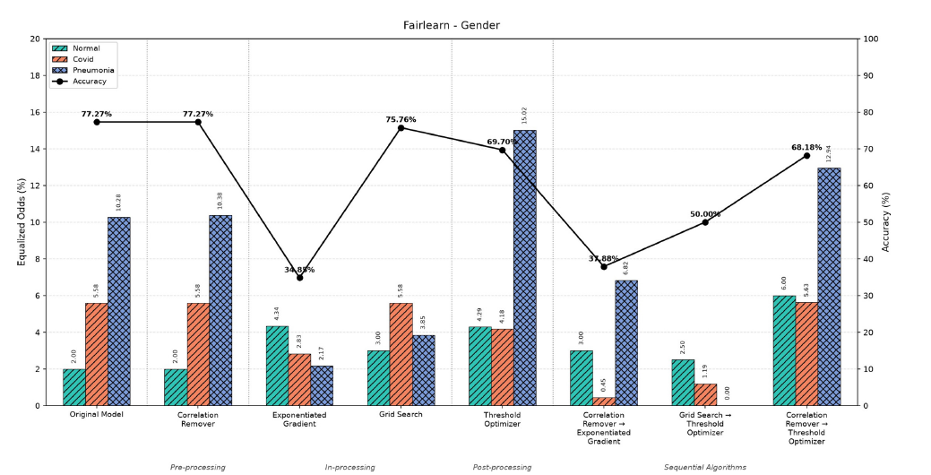
Figures 1&2 give the gender results. The untreated model is 77.27% accurate, with a largest DPD of 4.44% on viral pneumonia and a largest EOD of 10.28% on viral pneumonia. Of the three attributes, gender is the least affected, which leaves the mitigation algorithms the least room to work with.

Figure 1:Demographic parity difference per diagnosis, gender. Bars read against the left axis; the black line gives accuracy on the right. The zero for viral pneumonia under grid search followed by the threshold optimizer arises because that configuration no longer predicts the class.

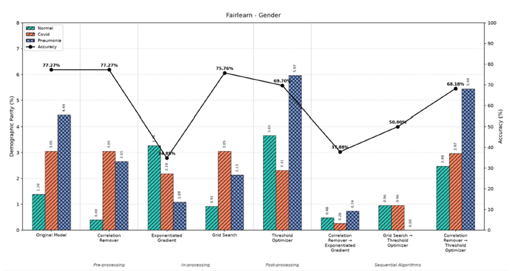
Figure 2:Equalized odds difference per diagnosis, gender. Grid search followed by the threshold optimizer brings the largest gap from 10.28% to 2.50%, the best gender result in the study, at 50.00% accuracy. The correlation remover followed by the threshold optimizer instead raises it to 12.94%.

For demographic parity, three of the four single-stage methods improve on the untreated model, and one does so for free. The correlation remover brings the DPD down to 3.05% (on Covid-19) at exactly 77.27% accuracy, no cost at all; grid search reaches the identical 3.05% but gives up 1.51 accuracy points to get there, so the correlation remover dominates it. The exponentiated gradient reduction reaches 3.26% but at an accuracy of only 34.85%. The threshold optimizer is the one method that makes things worse, pushing the DPD to 5.97% on viral pneumonia while holding accuracy at 69.70%. Chaining helps here in a way it does not elsewhere in this study: the correlation remover followed by the exponentiated gradient reduction cuts the DPD to 0.74%, the smallest value recorded for this attribute, though only at 37.88% accuracy.

For equalized odds the exponentiated gradient reduction gives the clearest single-stage improvement, taking the largest gap from 10.28% to 4.34% at 34.85% accuracy, with grid search a cheaper but smaller improvement at 5.58% for 75.76% accuracy. The correlation remover alone is not helpful, leaving the gap at 10.38%, marginally worse than untreated. Chaining again pays off on this attribute: grid search followed by the threshold optimizer reaches 2.50%, the best equalized-odds figure for gender in the whole study, at 50.00% accuracy. The threshold optimizer alone is the worst configuration tested for gender, raising the gap to 15.02% on viral pneumonia, with the correlation remover followed by the threshold optimizer next at 12.94% (Figures 1&2).

Ethnicity

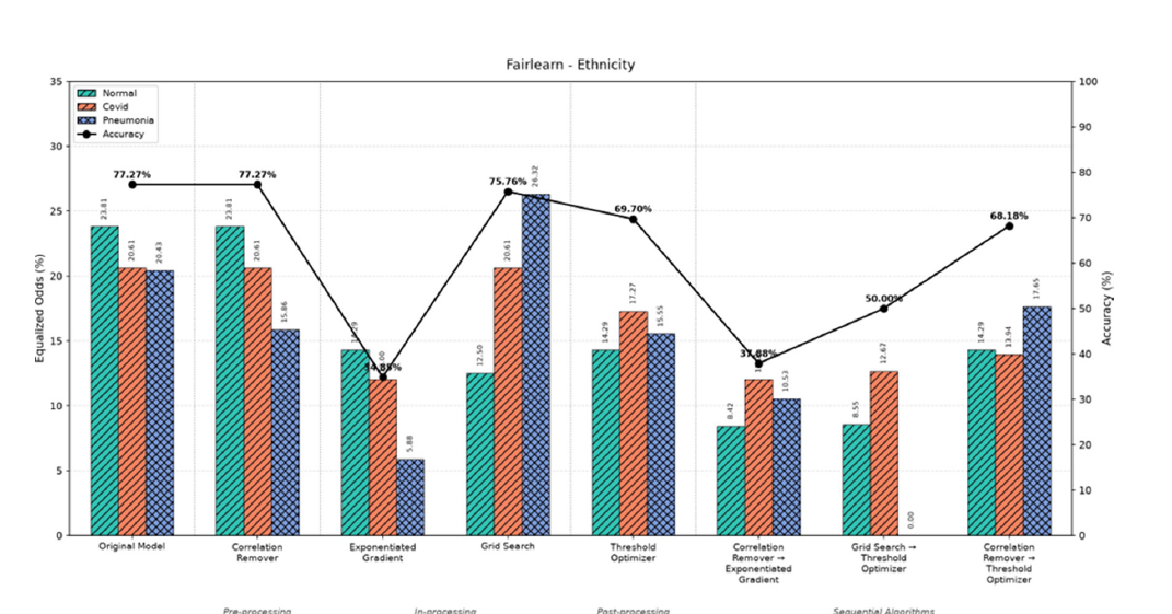
Figures 3&4 give the ethnicity results, and the gaps are wider than for gender: 10.75% for the largest DPD, on viral pneumonia and 23.81% for the largest EOD, on normal studies. Ethnicity is nonetheless the more affected of the two single attributes in this run. Since ethnicity here is assigned independently of image content by uniform random sampling (Section 4.3) rather than inferred from the pixels, this cannot be explained by the real-world finding that racial identity is recoverable from radiographs with near-perfect reliability [30,32] - that finding concerns a different kind of label than the one used here. We instead read the wider gap as reflecting how the classifier’s existing, unevenly distributed errors happen to interact with an unconditioned random partition into five groups rather than two, not as evidence that the model is responding to any demographic signal, real or simulated.

For demographic parity every single-stage method improves on the untreated 10.75%: the correlation remover reaches 10.14% at full accuracy, the exponentiated gradient reduction reaches 7.97% at 34.85% accuracy, the threshold optimizer reaches 9.88% at 69.70% accuracy, and grid search reaches 9.68%. This is the one panel in which every single-stage configuration improves on doing nothing. Chaining sharpens the best result further: grid search followed by the threshold optimizer reaches 6.25%, the narrowest ethnicity DPD recorded, at 50.00% accuracy.

For equalized odds the exponentiated gradient reduction again gives the largest single-stage improvement, from 23.81% to 14.29% at 34.85% accuracy, with the threshold optimizer a more moderate improvement to 17.27% at 69.70% accuracy. Grid search is the one method that makes the gap worse, reaching 26.32%. Chaining continues to help: the correlation remover followed by the exponentiated gradient reduction reaches approximately 12.00% and grid search followed by the threshold optimizer reaches 12.67%, both roughly halving the untreated gap. Unlike the previous run of this experiment, the ethnicity error-rate gap did yield to several of the methods applied here (Figure 3&4).

Figure 3:Demographic parity difference per diagnosis, ethnicity. Every single-stage method reaches or improves on the untreated 10.75%, and grid search followed by the threshold optimizer reaches 6.25%, the narrowest value recorded for this attribute.

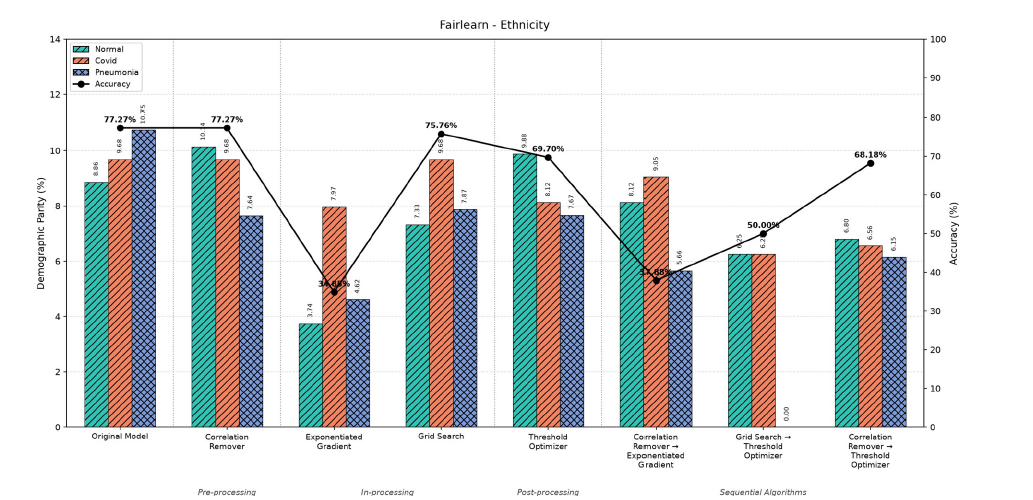
Figure 4:Equalized odds difference per diagnosis, ethnicity. The exponentiated gradient reduction brings the untreated 23.81% down to 14.29%, and chaining sharpens it further to roughly 12.00%. Grid search alone is the exception, raising the gap to 26.32% on viral pneumonia.

Subgroups defined by both attributes

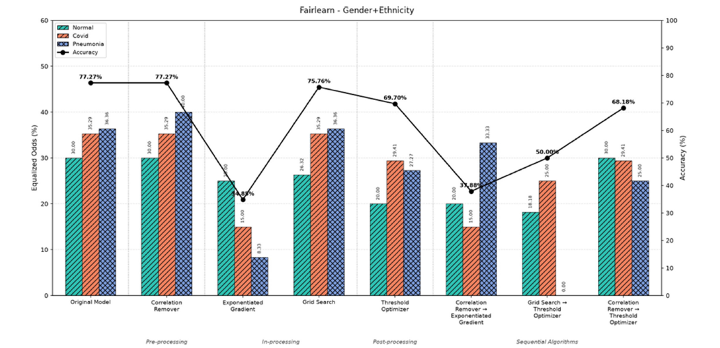
Figures 5&6 report subgroups defined by gender and ethnicity together, and the gaps are wider than for either attribute separately: 20.69% for the largest DPD, on Covid-19 and 36.36% for the largest EOD, on viral pneumonia, against 10.75% and 23.81% for ethnicity and 4.44% and 10.28% for gender. A model that looks tolerable on each attribute in isolation is not tolerable on the two together, which is the pattern that intersectional audits have repeatedly found [2,62].

For demographic parity, five of the seven mitigated configurations improve on the untreated value: the exponentiated gradient reduction and the correlation remover followed by the exponentiated gradient both reach 14.29%, the threshold optimizer and the correlation remover followed by it both reach 17.24%, and grid search followed by the threshold optimizer reaches 13.79%. The correlation remover alone ties the untreated value at 20.69% and grid search alone is the one method that worsens it, to 21.55%.

For equalized odds the exponentiated gradient reduction again leads the single-stage methods, taking the largest gap from 36.36% to 25.00% at 34.85% accuracy; grid search ties the untreated value exactly and the correlation remover is the one configuration that worsens it, to 40.00%, the widest gap recorded in the whole study. Chaining ties the single-stage result: grid search followed by the threshold optimizer also reaches 25.00%, at 50.00% accuracy, while the correlation remover followed by the threshold optimizer is more moderate, at 30.00%.

These figures should be read as approximate. Several of them are ratios of small whole numbers, which tells us that few patients fall into the individual combined subgroups. The ordering of configurations is worth attention; small differences between adjacent ones are not (Figures 5&6).

Figure 5:Demographic parity difference per diagnosis, subgroups defined by gender and ethnicity together. The expo-nentiated gradient reduction and grid search followed by the threshold optimizer both improve on the untreated 20.69%, the latter reaching 13.79%. Grid search alone reaches 21.55%.

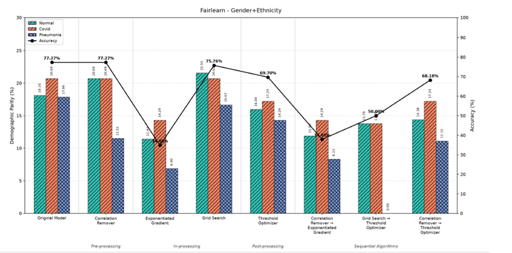
Figure 6:Equalized odds difference per diagnosis, subgroups defined by gender and ethnicity together. The untreated gap of 36.36% is the widest of the three attributes. The exponentiated gradient reduction and grid search followed by the threshold optimizer both bring it to 25.00%, while the correlation remover alone raises it to 40.00%, the widest gap recorded in the study.

Overview of the fairlearn results

Table 4 collects the best configuration of each type for every attribute and metric. In this run every one of the six rows has at least one entry, usually more than one, that beats the untreated model; the qualification is that the cheapest improvements (the correlation remover, and grid search) are modest, while the largest improvements come from the exponentiated gradient reduction and its chains, which routinely give up thirty to forty-five accuracy points to get there (Table 4).

Table 4:Best configurations measured with Fairlearn. All disparity values are the largest of the three per-class figures, in percentage points. The untreated model is 77.27% accurate.

Disparities Measured with AIF360

AIF360 takes the three-class problem directly, so no oneversus- rest split was needed and the figures are not per-class. Five metrics are reported. The first three compare a favoured subgroup with a disfavoured one:
1. The Statistical Parity Difference (SPD), the gap in how often a favourable outcome is issued, and the counterpart of demographic parity above;
2. The Average Odds Difference (AOD), the mean of the false positive and true positive rate gaps;
3. The Equal Opportunity Difference (EOD), the gap in detection rate alone, which is to say the gap in sensitivity.

The last two describe how unevenly the benefit of the model is spread across individual patients rather than across groups: the Theil index and the Generalized Entropy Index (GEI).

Privileged and unprivileged groups, and the favourable outcome

AIF360’s group-fairness metrics require a binary privileged/ unprivileged split and a definition of which predicted class counts as the favourable outcome. Reading the notebook, neither is a single fixed designation: for a given sensitive attribute, the code loops over every candidate category in turn, treats it as ”privileged” against all remaining categories pooled as “unprivileged,” computes the metric, and reports the maximum over all such choices - structurally the same one-vs-rest-and-take-the-maximum idea Fairlearn uses, just applied across subgroup categories rather than across diagnostic classes. Concretely: for gender, both categories are tried as privileged and the max taken. For ethnicity, four of the five categories (White, Black, Asian, Indian) are tried as privileged, each against the rest; Others is never tried as the privileged category, though it remains in the data and in the unprivileged pool. For the combined attribute, all eight (Gender × {White, Black, Asian, Indian}) cells are tried in turn, again excluding Others. The favourable outcome is the Covid diagnosis (favorable classes= [1]) in most of the mitigation sections, but the Learning Fair Representations step, which fits its own internal notion of favourable/unfavourable, instead treats Viral Pneumonia (favorable classes= [2]) as favourable. These choices are not neutral: which category is privileged in a given sweep determines the sign and because a maximum is then taken, potentially the size of every SPD, AOD and EOD value reported below and which class is coded favourable determines what ”favourable outcome” means for a three-way diagnostic decision where predicting Covid is not obviously more beneficial to a patient than predicting Normal.

Separately, the untreated (“Original”) model’s own baseline bias-identification computation - the reference point every mitigation configuration in this section is compared againstpreviously passed label name=‘Age’ to AIF360’s Standard Dataset, rather than label name=‘Status’ as every mitigation-algorithm section correctly did. Age is the independently generated, diagnosisirrelevant integer de-scribed in Section 4.3, not the diagnosis, and because the code treated values 0-2 as the favourable class, this produced a degenerate labeling in which no sample ever satisfied the favourable-class condition for the baseline computation alone. With label name set to ‘Status’ in all three baseline-metric cells, consistent with every mitigation configuration it is compared against, the SPD/AOD/EOD/Theil/GEI figures reported below come from the baseline computed against the true diagnostic label.

Eight algorithms were evaluated, covering all three points of intervention. Reweighing assigns training weights that decouple the label from the subgroup attribute [46]. The disparate impact remover edits feature values so that subgroup membership is harder to predict from them Feldman M, et al. [47]. Learning fair representations encodes the data in a form that retains diagnostic content while obscuring subgroup identity [60]. The exponentiated gradient and grid search reductions train under a fairness constraint, the first by iterative search and the second over a grid of constraint weights [49]. Equalized odds post-processing revises predictions until detection and false alarm rates match [51], its calibrated variant does so while preserving calibrated scores [52] and reject option classification revises only predictions falling near the decision boundary, in favour of the disfavoured group [53].

Figures 7-9 report all five metrics with accuracy. For the untreated model the three-subgroup metrics, in the order SPD, AOD, EOD, are 4.56%, 3.23%, and 3.30% for gender; 13.48%, 13.34%, and 10.40% for ethnicity; and 23.14%, 23.04%, and 20.69% for the two combined. The ordering agrees with Fairlearn: ethnicity is worse than gender and the combination worse than either.

Figure 7:AIF360 metrics and accuracy, gender. The untreated gaps are narrow, the disparate impact remover improves all three at a large accuracy cost, and equalized odds post-processing and reject option classification show the near-zero-disparity, near-30%-accuracy signature of a collapsed classifier.

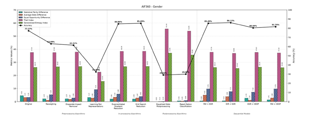
Figure 8:AIF360 metrics and accuracy, ethnicity. The exponentiated gradient reduction improves all three subgroup metrics while raising accuracy to 84.86%, and reweighing followed by the exponentiated gradient reduction improves on the untreated model at 85.49% accuracy, though not as narrowly as the exponentiated gradient reduction alone.

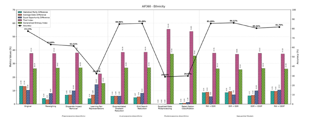
Figure 9:AIF360 metrics and accuracy, subgroups defined by gender and ethnicity together. Grid search reduction takes the EOD from 20.69% to 6.95% while raising accuracy to 85.49%; the two leading chains reach the same accuracy or higher (85.49% and 86.12%) but with wider gaps than their constrained-learner component alone.

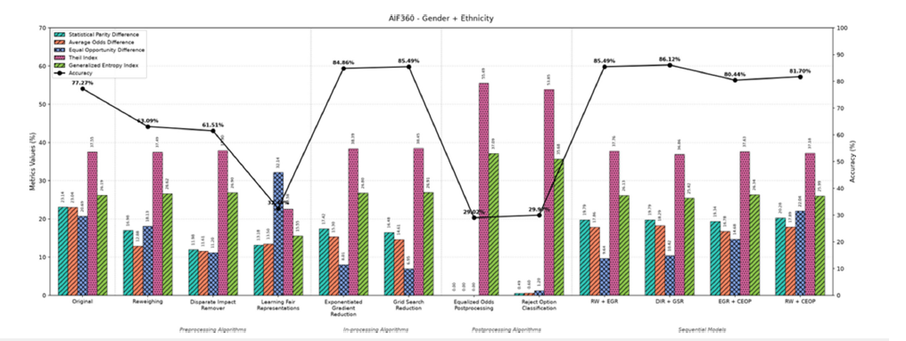
Two configurations need to be flagged before the rest are discussed, because they show the same signature as the collapsed Fairlearn configuration in Section 7.4. Equalized odds postprocessing returns SPD, AOD, and EOD values indistinguishable from zero for every attribute-0.03%/0.12%/0.24% for gender and 0.00%/0.00%/0.00% for both ethnicity and the combined attribute-at an accuracy of 29.02% and reject option classification is nearly as extreme, at 29.97% accuracy with every subgroup metric under 1.4%. An accuracy near 29% is close to the prevalence of the least common class in this corpus (Normal and Viral Pneumonia each make up 28.4% of the 317 images), which is consistent with a model that has stopped predicting the favourable Covid class altogether: with no favourable predictions issued to any subgroup, SPD, AOD and EOD are forced toward zero for the same structural reason the Fairlearn collapse forces its zero. We therefore read both configurations’ near-zero disparities as very likely artefacts of collapse rather than genuine correction, and flag them wherever they would otherwise appear to lead a comparison.

Single-stage algorithms

Setting the two apparently collapsed post-processing methods aside, the disparate impact remover is the strongest single-stage method in this run: for gender it takes SPD/AOD/EOD from 4.56%/3.23%/3.30%

to 2.25%/1.87%/2.84% and for the combined attribute from 23.14%/23.04%/20.69% to 11.98%/11.61%/11.20%, improving all three metrics for all three attributes at once-the only configuration in the study to do so-at a cost of 15.76 accuracy points (77.27% to 61.51%).

The two constrained learners are cheaper and nearly as effective. The exponentiated gradient reduction improves all three ethnicity metrics, to 5.93%, 6.04% and 6.00%, while raising accuracy to 84.86%, a genuine win-win rather than a trade. Grid search reduction does the same for the combined attribute, taking SPD/AOD/EOD from 23.14%/23.04%/20.69% to 16.48%/14.61%/6.95%-the EOD falling to roughly a third of its untreated value - while raising accuracy to 85.49%. Reweighing improves gender SPD and AOD but worsens EOD (3.30% to 5.28%) at a cost of 14.18 accuracy points and on the combined attribute it improves all three metrics only modestly. Learning fair representations is the least accurate of the remaining single-stage methods (32.49%) and is also one of the worst on disparity for the combined attribute, with an EOD of 32.14%, the widest subgroup-metric value recorded anywhere in the AIF360 half of this study.

Sequential algorithms

The chained configurations deliver the two highest accuracies in the study, but not the narrowest gaps. Reweighing followed by the exponentiated gradient reduction reaches an accuracy of 85.49%, above the untreated 77.27%, with subgroup metrics of 8.59%/8.94%/5.66% for ethnicity and 19.79%/17.86%/9.64% for the combined attribute - an improvement on the untreated model for every one of these six figures, though a smaller improvement than the exponentiated gradient reduction achieves on its own for ethnicity (5.93%/6.04%/6.00%). The disparate impact remover followed by grid search reduction delivers the highest accuracy anywhere in the study, 86.12%, with combined-attribute metrics of 19.79%/18.29%/10.42%, again an improvement on the untreated model but, again, not as narrow as grid search reduction achieves by itself (16.48%/14.61%/6.95%). The two chains ending in the calibrated variant of equalized-odds post-processing are more moderate: exponentiated gradient reduction followed by it reaches 80.44% accuracy with a combined EOD of 14.68% and reweighing followed by it reaches 81.70% accuracy with a combined EOD of 22.04%, the widest of the four chains.

Section 7.3 takes these two leading chains apart and asks which link is doing the work, since the comparison against the untreated model does not answer that question.

Inequality between individual patients

Unlike an earlier run of this experiment, the two individuallevel metrics moved substantially here. The untreated model has a Theil index of 37.55% and a GEI of 26.19%. Across the twelve configurations the Theil index ranges from 22.58% (learning fair representations) to 55.49% (equalized odds post-processing) and the GEI from 15.55% to 37.09% over the same two configurations. Both extremes belong to configurations already flagged above as unusual: learning fair representations is the least accurate genuine correction in the study and equalized odds post-processing is one of the two configurations we read as collapsed. Excluding those two and reject option classification, the other configuration we read as collapsed, the remaining nine configurations keep the Theil index within a narrower 36.86%-38.45% band and the GEI within 25.42%-26.91%, much closer to the untreated values and closer to the narrow range an earlier run of this experiment reported for all twelve.

The pattern therefore has to be read carefully: the wide overall range is driven by the configurations most likely to be pathological (a near-total loss of one output class, or a heavily obscured representation, both of which mechanically compress the diversity of predictions and can push an individual-level inequality measure in either direction), while the group-fairness-improving configurations that do not exhibit that signature leave individuallevel inequality close to where the untreated model left it. The two families of metric are still asking different questions, and an improvement in one is still not evidence of an improvement in the other [63,64], but in this run that dissociation is clearest precisely where a model has stopped behaving like a working classifier at all (Figures 7-9).

Overview of the AIF360 results

Table 5 separates the configuration with the narrowest gaps from the one that strikes the best balance of gap and accuracy, excluding the two apparently collapsed post-processing configurations from both columns. For ethnicity and for the combined attribute the two constrained learners, taken alone, are good enough to serve as both the narrowest-gap and a strong-balance entry, since each improves every subgroup metric while also raising accuracy; the sequential configurations deliver still higher accuracy but slightly wider gaps than their constrained-learner component achieves by itself (Table 5).

Table 5:Best configurations measured with AIF360, excluding equalized odds post-processing and reject option classification, both of which show the near-zero-disparity, near-30%-accuracy signature of a collapsed classifier (Section 6.2). Subgroup metrics are given as SPD / AOD / EOD in percentage points. The untreated model is 77.27% accurate with a Theil index of 37.55%.

Cross-Cutting Findings

Five findings emerge only when the nine figures are read against one another rather than one at a time.

More corrections helped this time, and displacement is harder to find

Summarising a configuration by its largest per-class gap conceals something the per-class figures reveal. Setting aside the collapsed configuration described below, thirty-six combinations of configuration and Fairlearn panel remain, and twenty-five of them improve on the untreated model, a substantially larger fraction than an earlier run of this experiment found. Five of those twentyfive keep the accuracy cost under two points, and all five belong to the correlation remover or grid search, the two single-stage methods that leave the model itself the least disturbed. Every one of the six panels now contains at least one improvement; none is shut out entirely, which was not true before.

We looked specifically for the kind of hidden displacement an earlier run of this experiment documented, where the largest perclass gap falls while the sum across all three classes rises. Checking all thirty-six non-untreated, non-collapsed configuration-and-panel combinations, we did not find a single instance of it here: wherever the largest per-class gap improved on the untreated model, the sum of the three per-class gaps improved alongside it and wherever the sum worsened, the largest gap had already worsened too. Displacement of totals behind a headline figure is therefore not a feature of this run, though we would not generalise from one run to a claim that it cannot occur.

What does still move is which diagnosis carries the widest gap and that continues to shift under mitigation just as it did before. In the gender demographic-parity panel the untreated model’s widest gap falls on viral pneumonia; it moves to Covid-19 under the correlation remover and under grid search and to normal studies under the exponentiated gradient reduction. In the combinedattribute demographic-parity panel the widest gap sits on Covid-19 for four of the seven mitigated configurations, moves to normal studies under grid search, and is shared equally between normal studies and Covid-19 under the correlation remover and under grid search followed by the threshold optimizer. An auditor who reports only the size of the largest gap, without naming which diagnosis it falls on, will describe a different clinical problem from one configuration to the next even when the number itself barely changes.

The sign of the accuracy relationship depends on whether collapsed configurations are included

We report this section as exploratory rather than confirmatory: the twelve configurations are not twelve independent draws, since the sequential configurations are built by applying a second algorithm to the output of a single-stage one, several share the same underlying constrained-learner code and all twelve are evaluated on the same held-out partition and the same single run of subgroup-label assignment (Section 8 discusses the singlerun limitation further). Correlating each AIF360 metric against accuracy across all twelve configurations gives a result dominated by the two configurations flagged in Section 6.2 as apparently collapsed: with equalized odds post-processing and reject option classification included, the combined-subgroup EOD correlates with accuracy at only r = +0.08, the combined SPD at r = +0.86, and the combined AOD at r = +0.82 - almost every criterion moving in the same direction as accuracy, which is the opposite of the usual fairness-accuracy trade-off and is driven by two configurations sitting at the extreme where both accuracy and every disparity metric collapse toward the same corner of the plot.

Excluding those two configurations changes the picture. Across the remaining ten, the combined-subgroup EOD correlates with accuracy at r = -0.75 and the ethnicity EOD at r = -0.77, both back in the direction the impossibility results would lead one to expect, while the ethnicity SPD correlates at r = +0.42 and the combined SPD at r = +0.67, positive but weaker than the error-rate criteria’s negative correlation. The sign of the headline correlation in this run therefore depends less on which fairness criterion is examined, as an earlier run of this experiment concluded, and more on whether the two apparently collapsed configurations are left in the sample: a practitioner computing this kind of correlation on a small set of configurations should check for a degenerate classifier hiding among them before reading the sign of the result as evidence about a fairness-accuracy trade-off at all.

The general caution nonetheless survives: the impossibility results discussed in Section 3.3 guarantee that not every criterion can be satisfied at once when base rates differ, but they do not by themselves guarantee the direction or size of any particular correlation. The criterion should still be chosen first, on clinical grounds, and the configuration chosen afterwards, with any correlation of this kind checked for the influence of degenerate configurations before it is used to argue that fairness must cost accuracy or that it does not.

Where the benefit of chaining comes from

Both AIF360 chains improve substantially over their untreated baseline, reweighing followed by the exponentiated gradient reduction reaching 85.49% accuracy against the untreated 77.27%, and the disparate impact remover followed by grid search reduction reaching 86.12%, the highest in the study. Read against the untreated model alone, the case for chaining looks straightforward.

Comparing each chain against its own constrained-learner component tells a more specific story, set out in Table 6. Adding the upstream repair improves the SPD only for gender, in both chains; it worsens the AOD in every one of the six attribute-andchain combinations; and it improves the EOD only for ethnicity, again in both chains, while worsening it for gender and for the combined attribute. Accuracy rises by a consistent 0.63 points in both chains, regardless of which attribute is being measured, since accuracy does not depend on which sensitive attribute the metrics are computed against.

The two stages therefore trade rather than accumulate: the upstream repair buys a real but narrow benefit (a lower gender SPD, a lower ethnicity EOD, and a small, uniform accuracy gain) at the cost of a worse AOD across the board and a worse gender and combined-attribute EOD. This is a more mixed picture than a simple story of “the constrained learner supplies fairness and the upstream stage supplies accuracy” would suggest, and it tells a practitioner specifically what is being traded rather than only that a chain performed well (Table 6).

Table 6:What the upstream stage adds, computed as each AIF360 chain minus its constrained learner alone. Negative values mean the subgroup metric improved. Accuracy rises by exactly 0.63 points in both chains, for every attribute, because accuracy does not depend on which sensitive attribute the disparity metrics are computed against.

Counting improvements across all nine attribute-and-metric cells gives another view, and here the disparate impact remover stands out: it improves all nine, the only genuine (non-collapsed) config-uration to do so, at a cost of 15.76 accuracy points. Reweighing improves eight of nine, and the exponentiated gradient reduction followed by calibrated equalized-odds post-processing improves eight of nine as well, and at no accuracy cost at all, since the exponentiated gradient reduction already raises accuracy on its own. If attention is narrowed to accuracy against combinedattribute EOD specifically, the configurations not dominated by any other are grid search reduction (6.95% EOD at 85.49% accuracy) and the disparate impact remover followed by grid search reduction (10.42% EOD at 86.12% accuracy, the highest accuracy in the study).

Two configurations that scored well by failing

Two collapses, one in each toolkit, can be accounted for exactly. Grid search followed by the threshold optimizer, in Fairlearn, reports identical or near-identical values for normal studies and for Covid-19 in the demographic-parity panels for every attribute-0.96%/0.96% for gender, 6.25%/6.25% for ethnicity, 13.79%/13.79% for the combined attribute-with viral pneumonia at exactly 0.00% in every case, at an accuracy of 50.00%. That coincidence is not a coincidence: if a model never returns viral pneumonia, the rate of predicting a normal study within any subgroup is one minus the rate of predicting Covid-19, so the two one-versus-rest parity gaps are forced to equality and the third is empty because there are no predictions of that class to compare.

In AIF360, equalized odds post-processing shows the equivalent signature from the opposite di-rection: SPD, AOD, and EOD all indistinguishable from zero for every attribute, at an accuracy of 29.02%, consistent with a model that has stopped predicting the favourable Covid-19 class rather than one of the unfavourable classes. Reject option classification, at 29.97% accuracy with every subgroup metric under 1.4%, shows a milder version of the same pattern. In both toolkits, an accuracy near the base rate of a single class, paired with near-zero disparity, is the signature to check for before reading a low disparity figure as a genuine correction.

Both episodes deserve reporting because any procedure that ranks configurations on group fairness alone, without also inspecting accuracy and the per-class or per-favourable-outcome structure behind it, would select one of these as among the fairest configurations tested. What each has actually done is stop making one kind of prediction altogether, which in a screening setting means an entire category of diagnostic outcome is denied to every subgroup equally. Equal treatment of this kind is not the goal the mitigation algorithms were applied to achieve.

The toolkits still contradicted one another

The sharpest disagreement in the study remains between the two pieces of software rather than between algorithms, though the size of the disagreement has narrowed. For ethnicity, Fairlearn records grid search raising the largest equalized odds gap from 23.81% to 26.32%, an increase of 10.5%. AIF360 records grid search reduction lowering the equal opportunity gap from 10.40% to 8.13%, a decrease of 21.8%. The accuracy attributed to the same nominal family of method differs by 9.73 points, 75.76% against 85.49%, smaller than before but still substantial for two runs of what is nominally the same algorithm. The two also disagree about the severity of the problem being solved, and this time in the opposite direction from before: Fairlearn puts the untreated combined-subgroup EOD at 3.54 times the gender figure (36.36% against 10.28%), while AIF360 puts it at 6.27 times (20.69% against 3.30%) - so where an earlier run found AIF360 understating the combined-subgroup penalty relative to Fairlearn, this run finds it overstating it.

Several things contribute, and they are not equally innocent, nor independent of one another. We separate them explicitly here rather than folding them into a single ”the toolkits disagree” statement:

1. Metric definition: Fairlearn’s equalized odds difference and AIF360’s equal opportunity difference are not the same quantity: the former is the larger of the true-positive-rate and false-positive-rate gaps, the latter is the true-positive-rate gap alone.
2. Multiclass decomposition: Fairlearn’s summary is a maximum over three one-versus-rest problems, one per diagnostic class. AIF360’s summary, we can now confirm from the notebook (Section 6.1), is also a maximum over one-versusrest problems, but taken across privileged-category choices for the sensitive attribute rather than across diagnostic classes, and taken over four or eight candidates (ethnicity, combined) rather than three. Both toolkits report a maximum over a onevs- rest sweep; they differ in what the sweep is over and how many candidates it has, not in whether one of them makes a single fixed comparison.
3. Implementation: The implementations differ, and this is not only qualitative: AIF360’s Grid Search Reduction here uses grid size=5, reduced from the library default of 10, while Fairlearn’s Grid Search uses grid size=40 (Section 4.2). An eightfold difference in how finely the constrained-optimisation grid is searched is a large, previously undisclosed asymmetry between the two “grid search” runs being compared, and is at least as plausible a source of the accuracy gap as anything about the two libraries’ internals in the abstract.
4. Model retraining: Because each toolkit’s grid search retrains the model independently rather than sharing weights or predictions, “the same intervention” here means the same nominal algo-rithm and hyperparameters, not the same trained model or the same predictions on the held-out set; we do not have matched per-example predictions from the two toolkits to test this directly.

The combined subgroups are also small, and several Fairlearn values are ratios of small whole numbers, which can exaggerate an apparent amplification independently of the four sources above. Sources 1 and 2 could in principle be neutralised by computing matched definitions on a single set of predictions, for example taking the class probabilities from one trained model and computing both a Fairlearn-style maximum-over-one-versus-rest gap and an AIF360-style privileged/unprivileged gap from them. Without that additional computation, the decomposition above should be read as an account of where the disagreement plausibly comes from, not as a demonstration that has isolated each source’s share; we accordingly avoid describing the two toolkits’ runs as “identical interventions” or “dentical predictions” elsewhere in the paper. The practical consequence is uncomfortable regardless of attribution: an audit of this classifier would conclude either that grid search narrows its ethnicity gap by a fifth or widens it by a tenth, depending on nothing but the choice of software. A disparity figure quoted without naming the toolkit that produced it claims more than the evidence supports.

Threats to Validity

Qualifications apply to everything above:

The subgroup labels are simulated rather than drawn from patient records, for the reason given in Section 4.3. Beyond that, they are not even fixed within this study: the assignment is unseeded, so the specific disparity documented above is one arbitrary draw rather than a deliberately structured, reproducible one. The figures reported here therefore describe how the mitigation methods behaved on a disparity that arose from independent random tabular features, on one run. They are not estimates of the disparity any deployed system exhibits, should not be cited as such, and would not be exactly reproduced by re-running the accompanying notebooks.

An earlier draft of this paper reported the untreated baseline in Section 6 from a mislabelled computation: the baseline biasidentification code used the diagnosis-irrelevant Age column rather than Status as the outcome label, while every mitigation configuration correctly used Status. This has since been corrected and the baseline re-run against Status (Section 6.1); the figures reported in Sections 6 and 7 reflect the corrected computation.

The combined subgroups are small. Several of the values reported for them are ratios of small whole numbers, so the ranking of configurations on that attribute carries more information than the individual figures do, and differences of two or three points between adjacent configurations should not be interpreted.

Each configuration was run once, and both reduction methods involve a randomised search over cost-sensitive subproblems; several intersectional subgroups are also small (Table 1), which com-pounds run-to-run variability for exactly the configurations whose combined-subgroup figures are emphasised in Sections 5.3 and 6. Repeated runs would vary, and small differences between neighbouring configurations may not survive replication.

Table 1 reports expected rather than observed subgroup counts. Because the gender and ethnicity assignment is unseeded and the run that produced the reported figures was not preserved, the per-run counts underlying those figures cannot be recovered, and the expected counts should not be used to verify any individual subgroup figure in Sections 5 and 6.

The comparison between the two toolkits is confounded by the differences in metric definition and implementation set out in Section 7.5. The disagreements reported there are properties of the software, not of the classifier, and we have been careful not to attribute them to the model.

Three practical constraints also shaped what could be attempted. Fairlearn does not accept three-class targets, so every metric had to be computed one class at a time and recombined by hand, which multiplies the number of figures an analyst must hold in view. Learning fair representations was the slowest method tested and would be impractical to tune on a local machine. And the reduction methods retrain the underlying model repeatedly, which caps the size of the search that fits in a fixed computational budget.

Conclusion

We set out to measure how unevenly a conventional chest radiograph classifier performs across patient subgroups and where in the pipeline that unevenness is best corrected. The model is 77.27% accurate, with equalized odds gaps of 10.28% for gender, 23.81% for ethnicity and 36.36% for both combined. AIF360 agrees on the ordering but puts the combined gap at 6.27 times the gender figure rather than 3.54 times, the reverse of an earlier run, so the toolkits disagree not just on magnitude but on which is more alarming, and an audit stopping at single attributes understates the problem.

Correction fared better than single-configuration reports in this literature suggest: 25 of 36 Fairlearn configuration-metric combinations improved on the untreated model, five at under two accuracy points of cost, and every panel admitted at least one improvement. We found no instance of the hidden displacement (a shrinking headline figure masking a growing total) an earlier run reported. What still shifts is which diagnosis carries the widest gap, changing at least once in every panel, so a single summary number remains misleading.

Three further findings stand out. Whether fairness appears to cost accuracy across the twelve AIF360 configurations depends less on the criterion than on whether two apparently collapsed configurations are included (r = +0.08 with them, r = -0.75 without), such correlations should be checked for degenerate configurations before their sign is trusted. Individual-level inequality moved substantially this time (Theil index 22.58%-55.49%), though most of that range comes from the three unusual configurations. And a disparity metric reached zero for the wrong reason twice, once per toolkit, each time by a model that stopped predicting one class rather than one that was genuinely corrected.

Chaining helped in both toolkits, but not by a clean division of labour: AIF360’s two leading chains reached the study’s highest accuracies (85.49%, 86.12%), while their upstream stages traded one metric for another rather than adding pure gains. Fairlearn’s chains also outperformed an earlier run, achieving the narrowest gender gaps in the study, though one did so by collapsing viralpneumonia predictions. Finally, the toolkits again reached opposite conclusions about the same nominal intervention, a 10.5% increase versus a 21.8% decrease for ethnicity, so no fairness figure should be quoted without naming the software behind it.

References

1. Madaio MA, Stark L, Vaughan JW, Wallach H (2020) Co-designing checklists to understand organizational challenges and opportunities around fairness in AI. Proceedings of the 2020 CHI Conference on Human Factors in Computing Systems, USA, pp: 1-14.
2. Buolamwini J, Gebru T (2018) Gender shades: Intersectional accuracy disparities in commercial gender classification. In Proceedings of the 1^st Conference on Fairness, Accountability and Transparency (FAT*), USA, pp: 77-91.
3. Guo A, Kamar E, Vaughan JW, Wallach H, Morris MR (2019) Toward fairness in AI for people with disabilities: A research roadmap. ArXiv.
4. Rudin C, Wang C, Coker B (2018) The age of secrecy and unfairness in recidivism prediction. ArXiv.
5. Aggarwal P, Mishra NK, Fatimah B, Singh P, Gupta A, et al. (2022) COVID-19 image classification using deep learning: Advances, challenges and opportunities. Computers in Biology and Medicine 144: 105350.
6. Krizhevsky A, Sutskever I, Hinton GE (2012) ImageNet classification with deep convolutional neural networks. Advances in Neural Information Processing Systems 25: 1097-1105.
7. Simonyan K, Zisserman A (2014) Very deep convolutional networks for large-scale image recognition. ArXiv.
8. He K, Zhang X, Ren S, Sun J (2016) Deep residual learning for image recognition. IEEE Conference on Computer Vision and Pattern Recognition (CVPR), USA, pp: 770-778.
9. Szegedy C, Liu W, Jia Y, Sermanet P, Reed S, et al. (2015) Going deeper with convolutions. IEEE Conference on Computer Vision and Pattern Recognition (CVPR), USA, pp: 1-9.
10. Chollet F (2017) Xception: Deep learning with depthwise separable convolutions. IEEE Conference on Computer Vision and Pattern Recognition (CVPR), USA, pp: 1800-1807.
11. Huang G, Liu Z, Maaten LVD, Weinberger KQ (2017) Densely connected convolutional networks. IEEE Conference on Computer Vision and Pattern Recognition (CVPR), USA, pp: 2261-2269.
12. Ronneberger O, Fischer P, Brox T (2015) U-Net: Convolutional networks for biomedical image segmentation. In International Conference on Medical Image Computing and Computer-Assisted Intervention (MICCAI), Springer, Cham, Switzerland, pp: 234-241.
13. Cohen JP, Morrison P, Dao L (2020) COVID-19 image data collection. Technical report, ArXiv.
14. Kermany D, Zhang K, Goldbaum M (2018) Labeled optical coherence tomography (OCT) and chest X-ray images for classification. Mendeley Data.
15. Abbas A, Abdelsamea MM, Medhat Gaber M (2021) Classification of COVID-19 in chest X-ray images using DeTraC deep convolutional neural network. Applied Intelligence 51(2): 854-864.
16. Ozturk T, Talo M, Yildirim EA, Baran Baloglu U, Yildirim O, et al. (2020) Automated detection of COVID-19 cases using deep neural networks with X-ray images. Computers in Biology and Medicine 121: 103792.
17. Wang L, Qiu Lin Z, Wong A (2020) COVID-Net: A tailored deep convolutional neural network design for detection of COVID-19 cases from chest X-ray images. Scientific Reports 10(1): 19549.
18. Iqbal Khan A, Latief Shah J, Mudasir Bhat M (2020) CoroNet: A deep neural network for detection and diagnosis of COVID-19 from chest X-ray images. Computer Methods and Programs in Biomedicine 196: 105581.
19. Rahimzadeh M, Attar A (2020) A modified deep convolutional neural network for detecting COVID-19 and pneumonia from chest X-ray images based on the concatenation of Xception and ResNet50V2. Informatics in Medicine Unlocked 19: 100360.
20. Oh Y, Park S, Chul Ye J (2020) Deep learning COVID-19 features on CXR using limited training data sets. IEEE Transactions on Medical Imaging 39(8): 2688-2700.
21. Narayanan BN, Hardie RC, Krishnaraja V, Karam C, Davuluru VSP (2020) Transfer-to-transfer learning approach for computer aided detection of COVID-19 in chest radiographs. AI 1(4): 539-557.
22. Tabik S, Gomez-Rios A, Martin-Rodriguez JL, Sevillano-Garcia I, Rey-Area M, et al. (2020) COVIDGR dataset and COVID-SDNet methodology for predicting COVID-19 based on chest X-ray images. IEEE Journal of Biomedical and Health Informatics 24 (12): 3595-3605.
23. Zhou B, Khosla A, Lapedriza A, Oliva A, Torralba A (2016) Learning deep features for discriminative localization. In: IEEE Conference on Computer Vision and Pattern Recognition (CVPR), USA, pp: 2921-2929.
24. Selvaraju RR, Cogswell M, Das A, Vedantam R, Parikh D, et al. (2017) Grad-CAM: Visual explanations from deep networks via gradient-based localization. In IEEE International Conference on Computer Vision (ICCV), Italy, pp: 618-626.
25. Chattopadhay A, Sarkar A, Howlader P, Balasubramanian VN (2018) Grad-CAM++: Generalized gradient-based visual explanations for deep convolutional networks. In IEEE Winter Conference on Applications of Computer Vision (WACV), USA, pp: 839-847.
26. Wang S, Kang B, Ma J, Zeng X, Xiao M, et al. (2021) A deep learning algorithm using CT images to screen for corona virus disease (COVID-19). European Radiology 31: 6096-6104.
27. Ardakani AA, Kanafi AR, Acharya UR, Khadem N, Mohammadi A (2020) Application of deep learning technique to manage COVID-19 in routine clinical practice using CT images: Results of 10 convolutional neural networks. Computers in Biology and Medicine 121: 103795.
28. DeGrave AJ, Janizek JD, Lee SI (2021) AI for radiographic COVID-19 detection selects shortcuts over signal. Nature Machine Intelligence 3: 610-619.
29. Karargyris A, Kashyap S, Wu JT, Sharma A, Moradi M, et al. (2019) Age prediction using a large chest X-ray dataset. Medical Imaging 2019: Computer-Aided Diagnosis 10950: 468-476.
30. Gichoya JW, Banerjee I, Bhimireddy AR, Burns JL, Anthony Celi L, et al. (2022) AI recognition of patient race in medical imaging: A modelling study. The Lancet Digital Health 4(6): e406-e414.
31. Duffy G, Clarke SL, Christensen M, He B, Yuan N, et al. (2022) Confounders mediate AI prediction of demographics in medical imaging. NPJ Digital Medicine 5(1): 188.
32. Liang H, Ni K, Balakrishnan G (2023) Visualizing chest X-ray dataset biases using GANs. Medical Imaging with Deep Learning (MIDL), ArXiv.
33. Karras T, Aittala M, Hellsten J, Laine S, Lehtinen J, et al. (2020) Training generative adversarial networks with limited data. Proceedings of the 34^th International Conference on Neural Information Processing Systems, USA, 33: 12104-12114
34. Karras T, Laine S, Aittala M, Hellsten J, Lehtinen J, et al. (2020) Analyzing and improving the image quality of StyleGAN. In IEEE/CVF Conference on Computer Vision and Pattern Recognition (CVPR), USA, pp: 8110-8119.
35. Irvin J, Rajpurkar P, Ko M, Yu Y, Ciurea-Ilcus S, et al. (2019) CheXpert: A large chest radiograph dataset with uncertainty labels and expert comparison. In: Proceedings of the Thirty-Third AAAI Conference on Artificial Intelligence and Thirty-First Innovative Applications of Artificial Intelligence Conference and Ninth AAAI Symposium on Educational Advances in Artificial Intelligence, USA, 33: 590-597.
36. Cohen JP, Brooks R, En S, Zucker E, Pareek A, et al. (2021) Gifsplanation via latent shift: A simple autoencoder approach to counterfactual generation for chest X-rays. In Medical Imaging with Deep Learning (MIDL), USA, pp: 74-104.
37. Singla S, Eslami M, Pollack B, Wallace S, Batmanghelich K (2023) Explaining the black-box smoothly-a counterfactual approach. Medical Image Analysis 84: 102721.
38. Dravid A, Schiffers F, Gong B, Katsaggelos AK (2022) medXGAN: Visual explanations for medical classifiers through a generative latent space. Computer Vision and Pattern Recognition (CVPR), pp: 2936-2945.
39. Seyyed-Kalantari L, Liu G, McDermott M, Chen IY, Ghassemi M (2021) CheXclusion: Fairness gaps in deep chest X-ray classifiers. In Pacific Symposium on Biocomputing, USA, 26: 232-243.
40. Wang X, Peng Y, Lu L, Lu Z, Bagheri M, et al. (2017) ChestX-Ray8: Hospital-scale chest X-ray database and benchmarks on weakly-supervised classification and localization of common thorax diseases. In: IEEE Conference on Computer Vision and Pattern Recognition (CVPR), USA, pp: 3462-3471.
41. Johnson AEW, Pollard TJ, Berkowitz SJ, Greenbaum NR, Lungren MP, et al. (2019) MIMIC-CXR, a de-identified publicly available database of chest radiographs with free-text reports. Scientific Data 6(1): 317.
42. Seyyed-Kalantari L, Zhang H, McDermott MBA, Chen IY, Ghassemi M (2021) Underdiagnosis bias of artificial intelligence algorithms applied to chest radiographs in under-served patient populations. Nature Medicine 27(12): 2176-2182.
43. Larrazabal AJ, Nieto N, Peterson V, Milone DH, Ferrante E (2020) Gender imbalance in medical imaging datasets produces biased classifiers for computer-aided diagnosis. Proceedings of the National Academy of Sciences 117(23): 12592-12594.
44. Glocker B, Jones C, Bernhardt M, Winzeck S (2023) Algorithmic encoding of protected characteristics in chest X-ray disease detection models. EBioMedicine 89: 104467.
45. Yi PH, Kim TK, Siegel E, Yahyavi-Firouz-Abadi N (2022) Demographic reporting in publicly available chest radiograph data sets: Opportunities for mitigating sex and racial disparities in deep learning models. Journal of the American College of Radiology 19(1): 192-200.
46. Kamiran F, Calders T (2012) Data preprocessing techniques for classification without discrimination. Knowledge and Information Systems 33(1): 1-33.
47. Feldman M, Friedler SA, Moeller J, Scheidegger C, Venkatasub-ramanian S (2015) Certifying and removing disparate impact. Proceedings of the 21^th ACM SIGKDD International Conference on Knowledge Discovery and Data Mining, USA, pp: 259-268.
48. Zhang BH, Lemoine B, Mitchell M (2018) Mitigating unwanted biases with adversarial learning. In AAAI/ACM Conference on AI, Ethics, and Society, USA, pp: 335-340.
49. Agarwal A, Beygelzimer A, Dudik M, Langford J, Wallach H (2018) A reductions approach to fair classification. Proceedings of the 35^th International Conference on Machine Learning, USA, 80: 60-69.
50. Kamishima T, Akaho S, Asoh H, Sakuma J (2012) Fairness-aware classifier with prejudice remover regularizer. In: Joint European Conference on Machine Learning and Knowledge Discovery in Databases (ECML PKDD), Springer, Germany, pp: 35-50.
51. Hardt M, Price E, Srebro N (2016) Equality of opportunity in supervised learning. Advances in Neural Information Processing Systems 29: 3315-3323.
52. Pleiss G, Raghavan M, Wu F, Kleinberg J, Weinberger KQ (2017) On fairness and calibration. Proceedings of the 31^st International Conference on Neural Information Processing Systems, USA, pp: 5684-5693.
53. Kamiran F, Karim A, Zhang X (2012) Decision theory for discrimination-aware classification. IEEE 12^th International Conference on Data Mining (ICDM), Belgium, pp: 924-929.
54. Kleinberg J, Mullainathan S, Raghavan M (2017) Inherent trade-offs in the fair determination of risk scores. In Innovations in Theoretical Computer Science (ITCS), USA.
55. Chouldechova A (2017) Fair prediction with disparate impact: A study of bias in recidivism prediction instruments. Big Data 5(2): 153-163.
56. Barocas S, Hardt M, Narayanan A (2023) Fairness and machine learning: Limitations and opportunities. MIT Press, USA.
57. Angwin J, Larson J, Mattu S, Kirchner L (2016) Machine bias: There’s software used across the country to predict future criminals. And it’s biased against blacks. ProPublica, USA.
58. Raikote P (2020) COVID-19 image dataset. Kaggle, USA.
59. Fairlearn, Software toolkit.
60. AI Fairness 360. Software toolkit, IBM.
61. Mittelstadt B, Wachter S, Russell C (2023) The unfairness of fair machine learning: Levelling down and strict egalitarianism by default. ArXiv.
62. Kearns M, Neel S, Roth A, Wu ZS (2018) Preventing fairness gerrymandering: Auditing and learning for subgroup fairness. Proceedings of the 35^th International Conference on Machine Learning (ICML), USA, pp:2564-2572.
63. Bellamy RKE, Dey K, Hind M, Hoffman SC, Houde S, et al. (2019) AI Fairness 360: An extensible toolkit for detecting, understanding, and mitigating un-wanted algorithmic bias. IBM Journal of Research and Development 63(4/5): 4:1-4:15.
64. Xu S, Strohmer T (2024) On the (in)compatibility between group fairness and individual fairness. ArXiv.