Analysis and Control of a Model Describing Food Insecurity and Disease Dynamics

Food insecurity and disease dynamics are part of a complex global web of interrelated social, economic, and environmental factors. Hunger and malnutrition weaken immune systems, increase vulnerability to infection, and worsen chronic diseases, while diseases themselves perpetuate poverty and food scarcity. The relationship is cyclical, creating a selfreinforcing trap that affects millions of people worldwide. To break this cycle, comprehensive strategies are needed-ones that integrate health, agriculture, and social protection policies while addressing the underlying causes of inequality and environmental degradation. Only through such coordinated efforts can humanity hope to achieve a world where every person enjoys both sufficient nourishment and the right to good health. Agusto [1] developed optimal chemoprophylaxis and treatment control strategies of a tuberculosis transmission model. Tien et al. [2], investigated multiple transmission pathways and disease dynamics in a waterborne pathogen model. Collins et al. [3] incorporated heterogeneity into the transmission dynamics of a waterborne disease model. Collins et al. [4], analyzed a waterborne disease model with socioeconomic classes. Collins et al. [5-7] performed computational work on waterborne and food-borne disease models.

Collins et al. [8] provided additional mathematical analyses of the effects of control measures in a waterborne disease model with socioeconomic conditions. Mugabi et al. [9] performed optimal control analysis of bluetongue virus transmission in patchy environments connected by host and wind-aided midge movements. Collins et al. [10] discussed the dynamics and control of mpox disease using two modelling approaches. Ibrahim et al. [11], discussed climate change, food security, and the attainment of sustainable development goals in Nigeria. Anggriani et al. [12] developed a mathematical model for a disease outbreak considering a waning-immunity class with nonlinear incidence and recovery rates.

Han et al. [13] discussed the associations between HbA1c and multiple diseases unveiled through a Mendelian randomization phenome-wide association study in East Asian populations. Collins et al. [14] developed optimal control strategies for reducing the interrelated issues of food insecurity and disease dynamics. In this work, bifurcation analysis and multi objective nonlinear model predictive control are performed on a dynamic model describing food insecurity and disease dynamics [14]. The paper is organized as follows. First, the model equations are presented, followed by a discussion of the numerical techniques involving bifurcation analysis and Multi objective Nonlinear Model Predictive Control (MNLMPC). The results and discussion are then presented, followed by the conclusions.

The scaled model Collins et al. [14] describing food insecurity and disease dynamics is presented in this section. The variables in the model, pv, qv, sv, iv, and yv, represent the scaled clean food resource variable, the scaled contaminated food resource variable, the scaled susceptible population, the scaled infected population, and the scaled food-secure population. All the variables are dimensionless. The control variables h1, h2, h3, h4, and h5 are the dimensionless control variables that represent purification measures, decrease in contact rates between safe food and contaminated food, treatment of infected individuals who are food insecure, job creation to create a decrease in food insecure populations, and proper disposal of unsafe food.

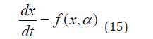
The model equations are

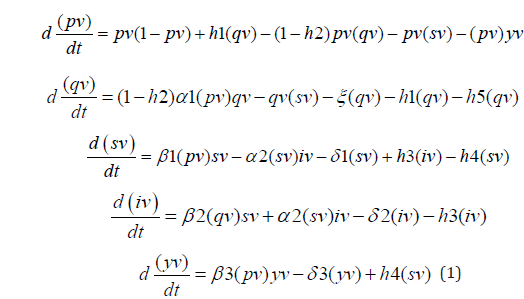
The other parameter values are α1 =0.0132; α 2 =0.1954; β1 =0.7508; β 2 =0.0108; β 3 =0.0110; ξ =0.1985; delta1 δ 1 =0.2099; δ 2 =0.0121; δ 3 =0.4996. These parameters are dimensionless and details of the derivations of the variables and parameters are presented in Collins et al. [14].

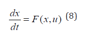
Bifurcation analysis deals with multiple steady-states (caused by branch and limit points) and limit cycles, which are caused by Hopf bifurcation points. The MATLAB program MATCONT (Dhooge Govearts & Kuznetsov [15]; Dhooge Govearts, Kuznetsov, Mestrom & Riet [16]) is used to locate limit points, branch points, and Hopf bifurcation points. In ODE system

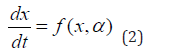
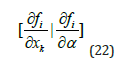
x ∈ Rⁿ Let the bifurcation parameter be α . Since the gradient is orthogonal to the tangent vector,

The tangent plane is the n+1-dimensional vector w that satisfies

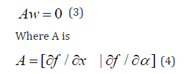
And ∂f / ∂x is the Jacobian matrix. For both limit and branch points, the Jacobian matrix J = [∂f / ∂x] must be singular.

For a limit point, there is only one tangent at the point of singularity. At this singular point, there is a single non-zero vector, y, where Jy=0. This vector is of dimension n. Since there is only one tangent the vector

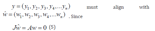
the n+1th component of the tangent vector w_n+1= 0 at a Limit Point (LP).

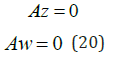
For a branch point, there must exist two tangents at the singularity. Let the two tangents be z and w. This implies that

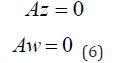
Consider a vector v that is orthogonal to one of the tangents (say w). v can be expressed as a linear combination of z and w ( v =α z +β w). Since Az = Aw = 0 ; Av = 0 and since w and v are orthogonal,

w^Tv = 0 . Hence 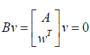which implies that B is singular.

Hence, the matrix is singular at a branch point.

When there is a Hopf bifurcation point the bialternate product,

where Jn is the n-square identity matrix. Hopf bifurcations cause limit cycles and should be eliminated because limit cycles make optimization and control tasks very difficult. More details can be found in Kuznetsov [17,18] and Govaerts [19]. Hopf bifurcations cause limit cycles. Limit cycles cause equipment damage and make control tasks difficult. Additionally, they result in less beneficial products. The tanh activation function (where a control value v is modified to (v tanh v /ε ) is used to eliminate spikes in profiles Dubey et al. [20]; Kamalov et al. [21] & Szandała, [22]; Sridhar [23,24] demonstrates with several examples how the activation factor involving the tanh function successfully eliminates the limit cycle causing Hopf bifurcation points by increasing the oscillation time period in the limit cycle.

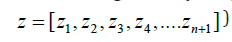
The rigorous Multiobjective Nonlinear Model Predictive Control (MNLMPC) method developed by Flores-Tlacuahuaz et al. [25] was used. Consider a problem where the variables have to be optimized together for a dynamic problem

t_f being the final time value and u the control parameter. The individual objective optimal control problem is solved by optimizing each of the variables The optimization of will lead to the values q_j∗. Then the Multiobjective Optimal Control (MOOC)problem

is solved. This will provide the value of u at each time step. The first obtained control value of u is implemented and this procedure is repeated until the implemented and the first obtained control values are the same or where ( for all j. Utopia point) is obtained.

The optimization program PYOMO Hart et al. [26] is used. Here, the differential equations are converted to a nonlinear program (NLP) using the orthogonal collocation method. The NLP is solved using IPOPT Wächter A & Biegler [27] and confirmed as a global solution with BARON Tawarmalani M & N Sahinidis [28].

The steps of the algorithm are as follows
1. Optimize and obtain q_j∗. 2. Minimize 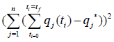and get the control values at various times. 3. Implement the first obtained control values 4. Repeat steps 1 to 3 until there is an insignificant difference between the implemented and the first obtained value of the control variables or if the Utopia point is achieved. The Utopia point is when 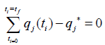for all j.

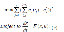
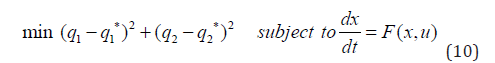
Sridhar [29] demonstrated that when the bifurcation analysis revealed the presence of limit and branch points the MNLMPC calculations to converge to the Utopia solution. For this, the singularity condition, caused by the presence of the limit or branch points was imposed on the co-state equation Upreti [30]. If the minimization of q₁ lead to the value q₁∗ and the minimization of q₂ lead to the value q₂∗ The MNLPMC calculations will minimize the function (q₁−q₂∗)² + (q₂−q₂∗)². The multiobjective optimal control problem is

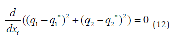
Differentiating the objective function results in

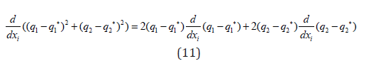
The Utopia point requires that both (q₁−q₁*) and 2 2 (q₂−q₂*) are zero. Hence

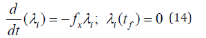
The optimal control co-state equation Upreti [30] is

λ_i is the Lagrangian multiplier. t_f is the final time. The first term in this equation is 0 and hence

At a limit or a branch point, for the set of ODE 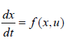is singular. Hence there are two different vectors-values for [λ_i] whe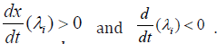re . In between there is a vector [λ_i] where . This coupled with the boundary condition will lead to This makes the problem an unconstrained optimization problem, and the optimal solution is the Utopia solution.

Theorem

If one of the functions in a dynamic system is separable into two distinct functions, a branch point singularity will occur in the system.

Proof

Consider a system of equations

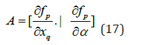
x ∈ Rⁿ . Defining the matrix A as

is the bifurcation parameter. The matrix A can be written in a compact form as

The tangent at any point 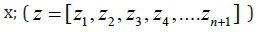must satisfy

The matrix must be singular at both limit and branch points... The n+1^th component of the tangent vector at a Limit Point (LP) and for a Branch Point (BP) the matrix must be singular. Any tangent at a point y that is defined by must satisfy

For a branch point, there must exist two tangents at the singularity. Let the two tangents be z and w. This implies that

Consider a vector v that is orthogonal to one of the tangents (say z). v can be expressed as a linear combination of z and w ( v =α z +β w). Since Az = Aw = 0 ; Av = 0 and since z and v are orthogonal, z^T v = 0 . Hence 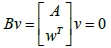which implies that B is singular where

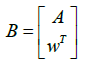
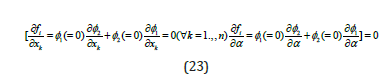
Let any of the functions fi are separable into 2 functions φ₁ ,φ₂ as

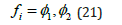
At steady-state f_i(x,α) =0 and this will imply that either φ₁ = 0 or φ₂ = 0 or both φ₁ and φ₂ must be 0. This implies that two branches φ₁ = 0 and 2 0 φ = will meet at a point where both φ₁ and φ₂ are 0.

At this point, the matrix B will be singular as a row in this matrix would be

However,

This implies that every element in the row , and hence the matrix B would be singular. The singularity in B implies that there exists a branch point.

Bifurcation Results

When bifurcation analysis is performed with α1 is the bifurcation parameter a branch point and a Hopf bifurcation point ) is found for (pv, qv, sv, iv, yv, α1 ) values of ( 0.938076, 0, 0.061924, 2.530232, 0, 0.277615 ) and (0.860319, 0.077876, 0.061805, 2.231460, 0, 0.302568). (Figure 1a) The limit cycle for this Hopf bifurcation is shown in (Figure 1b). When α1 is modified to (α1(tanh(α1)) / 0.001 the Hopf bifurcation disappears (Figure 1c) validating the analysis of Sridhar [24] The branch point occurs at (pv, qv, sv, iv, yv, α1) values of (0.938076, 0, 0.061924, 2.530232, 0, 0.277615). Here, the two distinct functions can be obtained from the second ODE in the model

Figure 1a:Bifurcation analysis (α1) .

Figure 1b:Limit cycle (α1)

Figure 1c:Hopf disappears when when (α1) is modified to (α1(tanh(α1)) / 0.001 .

Figure 1d:(h3 is bifurcation parameter).

Figure 1e:h4 is the bifurcation parameter.

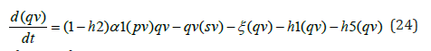
The two distinct equations are

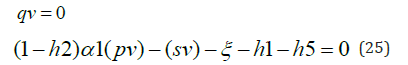
With qv=0, h2=h5=h1=0; and pv=0.938076, sv= 0.061924, =0.1985, both distinct equations are satisfied, validating the theorem.

When h3 is the bifurcation parameter, a branch point was found at (pv, qv, sv, iv, yv, h3) values of (0.279568; 0; 0.720432; 0; 0; 0.128672) (Figure 1d)

When h4 is the bifurcation parameter, a branch point was found at (pv, qv, sv, iv, yv, h4) values of (0.880999, 0, 0.061924, 0, 0.057076, 0.451554) and (1, 0, 0, 0, 0, 0.540900) (Figure 1e).

For the MNLMPC, h1, h2, h3, h4, h5 are the control parameters, and 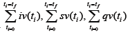were minimized individually, and each led to a value of 0. The overall optimal control problem will involve the minimization of 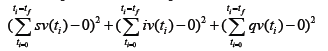was minimized subject to the equations governing the model. This led to a value of zero (the Utopia point). The MNLMPC values of the control variables, h1, h2, h3, h4, h5 were 0.04414, 0.473, 0.2373, 0.07865, 0.04413. The MNLMPC profiles are shown in (Figure 2a- 2d). The control profiles (h1, h2, h3, h4, h5) exhibited noise (Figure 2c). This was remedied using the Savitzky-Golay filter to produce the smooth profiles h1sg, h2sg, h3sg, h4sg, h5sg, (Figure 2d). The presence of the branch point causes the MNLMPC calculations to attain the Utopia solution, validating the analysis of Sridhar [29].

Figure 2a:MNLMPC sv,qv,iv.

Figure 2b:MNLMPC pv, yv.

Figure 2c:h1, h2, h3, h4, h5.

Figure 2d:h1sg, h2sg, h3sg, h4sg, h5sg.

Bifurcation analysis and Multiobjective Nonlinear Control (MNLMPC) studies on a model describing food insecurity and disease dynamics. The bifurcation analysis revealed the existence of a Hopf bifurcation point, and branch points. The Hopf bifurcation point, which causes an unwanted limit cycle, is eliminated using an activation factor involving the tanh function. The branch points (which cause multiple steady-state solutions from a singular point) are very beneficial because they enable the Multiobjective nonlinear model predictive control calculations to converge to the Utopia point (the best possible solution) in the models. A combination of bifurcation analysis and Multiobjective Nonlinear Model Predictive Control (MNLMPC) for a model describing food insecurity and disease dynamics is the main contribution of this paper.

1. Agusto FB (2009) Optimal chemoprophylaxis and treatment control strategies of a tuberculosis transmission model. World J Model Simul 5: 163-173.
2. Tien JH, Earn DJD (2010) Multiple transmission pathways and disease dynamics in a waterborne pathogen model. Bull Math Biol 72(6): 1506-1533.
3. Collins OC, Govinder KS (2014) Incorporating heterogeneity into the transmission dynamics of a waterborne disease model. J Theor Biol 356: 133-143.
4. Collins OC, Robertson SL, Govinder KS (2015) Analysis of a waterborne disease model with socioeconomic classes. Math Biosci 269: 86-93.
5. Collins OC, Govinder KS (2016) Stability analysis and optimal vaccination of a waterborne disease model with multiple water sources. Nat Resour Model 29 (3): 426-447.
6. Collins OC, Duffy KJ (2016) Consumption threshold used to investigate stability and ecological dominance in consumer-resource dynamics. Ecol Model 319 155-162.
7. Collins OC, Duffy KJ (2016) Optimal control of maize foliar diseases using the plant population dynamics. Acta Agric Scand Sect B Soil Plant Sci 66 (1): 20-26.
8. Collins OC, Duffy KJ (2021) Mathematical analyses on the effects of control measures for a waterborne disease model with socioeconomic conditions. J Comput Biol 28 (1): 19-32.
9. Mugabi F, Duffy KJ, Mugisha JY, Collins OC (2022) Optimal control analysis of bluetongue virus transmission in patchy environments connected by host and wind-aided midge movements. J Appl Math Comput 68 (3): 1949-1978.
10. Collins OC, Duffy KJ (2024) Dynamics and control of mpox disease using two modelling approaches. Model Earth Syst Environ 10 (2): 1657-1669.
11. Ibrahim AL, Ibrahim MS (2024) Climate change, food security and the attainment of sustainable development goals in Nigeria. J Political Discourse 2 (1): 45-57.
12. Anggriani N, Beay LK, Ndii MZ, Inayaturohmat F, Tresna ST (2024) A mathematical model for a disease outbreak considering the waning-immunity class with nonlinear incidence and recovery rates. J Biosaf Biosecurity 6 (3): 170-180.
13. Han L, Xu S, Chen R, Zheng Z, Ding Y, et al. (2025) Causal associations between HbA1c and multiple diseases unveiled through a mendelian randomization phenome-wide association study in east Asian populations. Medicine (Baltimore) 104(11): e41861.
14. Collins OC, KJ Duffy (2026) Optimal control strategies for reducing the interrelated issues of food insecurity and disease dynamics: A mathematical modelling approach using Nigeria as a case study. Comput Biol Chem 120 (Pt 1): 108664.
15. Dhooge A, Govearts W, Kuznetsov AY (2003) MATCONT: A matlab package for numerical bifurcation analysis of ODEs. ACM Transactions on Mathematical Software 29(2): 141-164.
16. Dhooge A, W Govaerts, YA Kuznetsov, W Mestrom, AM Riet, et al. (2004) MATCONT and CL MATCONT: A continuation toolbox in MATLAB 161-166.
17. Kuznetsov YA (1998) Elements of applied bifurcation theory. Springer, USA.
18. Kuznetsov YA (2009) Five lectures on numerical bifurcation analysis. Utrecht University, Netherlands.
19. Govaerts WJF (2000) Numerical methods for bifurcations of dynamical equilibria. SIAM, USA.
20. Dubey SR, Singh SK, Chaudhuri BB (2022) Activation functions in deep learning: A comprehensive survey and benchmark. Neurocomputing 503: 92-108.
21. Kamalov F, Nazir A, Safaraliev M, Cherukuri AK, Zgheib R (2021) Comparative analysis of activation functions in neural networks. 28^th IEEE International Conference on Electronics, Circuits, and Systems (ICECS) Dubai, United Arab Emirates, pp. 1-6.
22. SzandałaT (2020) Review and comparison of commonly used activation functions for deep neural networks. ArXiv.
23. Sridhar LN (2023) Bifurcation analysis and optimal control of the tu­mor macrophage interactions. Biomed J Sci & Tech Res 53(5): 45218-45225.
24. Sridhar LN (2024) Elimination of oscillation causing hopf bifurcations in engineering problems. Journal of Applied Math 2(5).
25. Tlacuahuac AF, Pilar M, Martin RT (2012) Multiobjective nonlinear model predictive control of a class of chemical reactors. I & EC Research 51(17): 5891-5899.
26. Hart WE, Carl DL, Jean PW, David LW, Gabriel AH, et al. (2017) Pyomo optimization modeling in python. (2^nd edn), Springer Nature, USA.
27. Wächter A, Biegler L (2006) On the implementation of an interior-point filter line-search algorithm for large-scale nonlinear programming. Math Program 106: 25-57.
28. Tawarmalani M, Sahinidis NV (2005) A polyhedral branch-and-cut approach to global optimization. Mathematical Programming 103(2): 225-249.
29. Sridhar LN (2024) Coupling bifurcation analysis and multiobjective nonlinear model predictive control. Austin Chem Eng. 11(1): 1-7.
30. Upreti SR (2013) Optimal control for chemical engineers. (1^st edn), Taylor and Francis, USA, p. 305.