Hydrodynamic Simulation of the Pineios River During the Daniel Flood Using the Delft3DFLOW Model

This study reconstructs the September 2023 Storm Daniel flood along the lower Pineiós (Pinios) River in Thessaly, Greece, using the Delft3D-FLOW hydrodynamic model. A three-dimensional σ-coordinate grid, incorporating available bathymetric surveys and interpolated channel geometry, was forced with ERA5 atmospheric reanalysis to simulate river–floodplain dynamics under the extreme rainfall of 5-7 September. A Python-based workflow was implemented to process meteorological fields and generate spatially and temporally consistent model inputs. To assess model performance, the inundation extent was compared with Copernicus Emergency Management Service (EMS) Rapid Mapping products. A structured geospatial preprocessing pipeline, combining reprojection, grid-based clipping, channel removal and polygon intersection, ensured spatial alignment between model outputs and EMS observations. Validation metrics demonstrate strong agreement, with Success Rates exceeding 0.94, low Failure Rates, and Centroid Skill Scores close to unity for both upstream and downstream sectors. The spatial patterns of inundation reflect the shift from narrow valley sections to the broader floodplain areas of northeastern Thessaly, matching independently mapped impacts of Storm Daniel. The results highlight the capability of Delft3D-FLOW to simulate extreme flood events in data-limited basins and provide a reproducible framework for integrating atmospheric reanalysis with high-resolution hydrodynamic modelling to support flood hazard assessment and regional resilience planning.

Keywords:Hydrodynamic modelling; Delft 3D-FLOW; Storm daniel; Flood mapping; Copernicus EMS; Thessaly

Rivers play a critical role in transporting water, sediments, and nutrients across landscapes, but they are also highly dynamic systems that can generate destructive flood events when extreme hydrological or meteorological conditions occur [1]. Floods may arise from excessive rainfall, dam failures, snowmelt, storm surges, or river channel overflow, often resulting in severe socio-economic and environmental impacts [2,3]. Understanding flood behavior through hydrodynamic modeling is therefore essential for hazard assessment, infrastructure planning and risk mitigation, particularly in regions where climate change is amplifying the frequency and intensity of extreme events [4,5].

Hydrodynamic models are indispensable tools for simulating and understanding flood propagation in riverine systems. Among these, Delft3D-FLOW has emerged as a widely used and reliable modeling framework for both two-dimensional and three-dimensional flow simulations [6]. The model solves the shallow water equations, incorporating key processes such as advection, diffusion, turbulence and bed friction, which enables accurate prediction of water levels, velocities and inundation extents under complex hydraulic conditions [7]. Its flexibility in handling variable topography, boundary conditions and flow scenarios makes it particularly suitable for simulating extreme events, including dam-breaks and storm-induced floods [8].

Delft3D-FLOW is particularly effective for simulating floods in rivers and estuarine environments due to its ability to resolve both hydrodynamics and water level variations under complex bathymetry. In estuaries, tidal interactions, freshwater inflows, and storm surges create highly variable water levels, which can be accurately captured using the model’s 3D hydrodynamic module [9]. For flood modeling, Delft3D-FLOW allows the simulation of extreme events, including dam-breaks and heavy rainfall-induced river floods, by solving the shallow water equations with explicit treatment of bed friction, turbulence and wetting-drying processes [10]. Its nested grid capability enables high-resolution modeling in areas of interest, such as urban floodplains or estuarine bottlenecks, while maintaining computational efficiency in larger domains [11].

In early September 2023, Storm Daniel unleashed extreme rainfall across central Greece, triggering catastrophic flooding in the plain of Thessaly. In the area of Larissa, the river Pinios River rose to around 9.5m, far exceeding normal levels, causing rapid overflow and inundation of the city’s northern districts and adjacent agricultural lands [12]. Satellite based mapping found that the flooding extended over approximately 355km2 in the Larissa regional unit alone, representing about 37% of the total inundated area in Thessaly. The event decimated infrastructure, disrupted transport networks and agricultural production, and underscored the urgent need for advanced hydrodynamic modeling to support flood risk management efforts in the region [13,14].

This study focuses on the Daniel flood event in Larissa, central Greece, which occurred in September 2023. The flood was triggered by extreme rainfall associated with Storm Daniel, causing rapid river discharge, overflow of the Pinios River, and extensive inundation of urban and agricultural areas. Accurate simulation of such extreme events is critical for flood risk assessment and management.

The objectives of this study are to:
A. Simulate flood propagation and inundation in the Larissa region using the Delft3D-FLOW model under observed extreme rainfall conditions.
B. Integrate realistic atmospheric forcing by incorporating ERA5 reanalysis data for rainfall and other meteorological parameters.
C. Develop a replicable workflow for converting ERA5 outputs into Delft3D-compatible input files to enable accurate and efficient hydrodynamic simulations.

This workflow allows researchers and practitioners to reproduce the approach for other riverine and estuarine floodprone regions, improving the realism and accuracy of simulations to support flood hazard assessment, emergency planning, and risk mitigation strategies.

This section provides a detailed overview of the hydrodynamic modeling approach applied to the Daniel flood in the region of Larissa, Greece. We begin by introducing the study area and outlining the key geographical and hydrological characteristics that contributed to the severity of the flood. Next, we present the governing equations that form the basis of the Delft3DFLOW simulations employed in this work. The development and validation of the computational grid are then described to ensure numerical stability and spatial accuracy throughout the domain. Finally, we outline the processing, configuration and integration of ERA5 atmospheric reanalysis data, which supply the rainfall and boundary conditions used as meteorological forcing for the hydrodynamic model.

Case study area

Fgure 1:Map of the Pinios river basin study area.

The case study focuses on the Pinios River Basin in central Greece, where the Daniel flood caused widespread inundation across the Thessaly plain, the country’s most productive agricultural region. The Pinios River (Figure 1) originates in the Pindus Mountains and flows eastward through Thessaly before draining into the Aegean Sea, forming a delta rich in riparian and coastal ecosystems.

The region is environmentally sensitive and designated as a Nitrate Vulnerable Zone (NVZ) under the EU Nitrates Directive. Consistent findings from long-term monitoring show extensive groundwater over-extraction, degradation of water quality, and elevated nitrogen contamination due to intensive agriculture and fertilizer application [15,16]. Despite agricultural pressures inland, nutrient loading at the coastal zones remains balanced, largely due to significant denitrification in groundwater, river sediments, ditches, and canals. As a result, eutrophication risk in the Pinios delta and coastal waters remains low [17]. Nevertheless, multiple studies consistently indicate that both surface and groundwater resources in the basin are highly vulnerable to nitrate pollution, over-abstraction, and contamination from agricultural practices [18,19].

Governing equations

The three-dimensional equations governing free-surface flows can be derived from the Navier-Stokes equations after averaging over turbulence time scales, resulting in the Reynolds-Averaged Navier-Stokes (RANS) equations. These equations express the fundamental principles of conservation of mass, momentum, and volume [6,20]. For many practical applications in rivers, estuaries and shallow coastal waters, the flow depth is small compared to horizontal length scales, which allows the use of the shallow water equations. Under the assumption that vertical accelerations are negligible relative to horizontal ones, the vertical momentum equation reduces to the hydrostatic pressure relation:

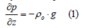
where: p = pressure, ρ_ο = the reference water density and g = gravity acceleration.

To account for flows over variable bathymetry, the vertical coordinate is transformed into a terrain-following σ-coordinate system, where σ = 0 at the free surface and σ = −1 at the bed. In this coordinate system, the three-dimensional hydrostatic shallow water equations can be expressed in Cartesian coordinates horizontally and σ-coordinates vertically. The horizontal momentum equations in the σ-coordinate system are:

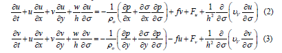
where: u, υ, w = the velocity components in the x, y and σ directions respectively, h = the total water depth, f = the Coriolis parameter accounting for Earth’s rotation, F_u, F_υ = horizontal viscosity terms, υ_V = the vertical eddy viscosity.

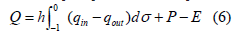
The continuity equation (mass conservation) is:

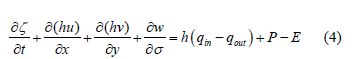
where: q_in and q_out = local water source and sink terms per unit volume (e.g., river inflows, withdrawals), P and E denote precipitation and evaporation fluxes at the surface.

The vertical velocities w in the σ-coordinate system is computed from the continuity equation:

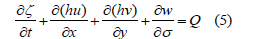
where: Q represents the net contributions per unit area from discharge, withdrawal, precipitation and evaporation, defined as:

The horizontal viscosity terms F_u, F_υ, representing turbulent momentum fluxes, are expressed as:

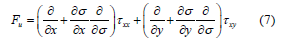
where: the Reynolds stresses τ_xx, τ_xy and τ_yy are parameterized using the Boussinesq approximation:

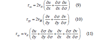
where: v_H = horizontal eddy viscosity coefficient.

Grid and independence tests

Grid generation is a key step in configuring hydrodynamic simulations in Delft3D-FLOW, as the computational mesh determines the spatial resolution and numerical framework over which water levels, velocities, and flood propagation are simulated. In riverine and estuarine environments, a well-constructed grid is essential to accurately represent channel geometry, floodplain topography and coastal interactions [6,21].

For the Pinios River and its deltaic outlet, the first stage involved defining the full spatial extent of the study area, including the main river channel, adjacent low-lying floodplain, and the estuarine transition to the Aegean Sea. Using Delft3D’s RGFGRID tool, the model boundaries were generated to follow the natural morphology of the riverbanks and coastline, ensuring smooth numerical representation of the terrain. Bathymetric data [22] were incorporated through Open Land Boundaries and Open Samples, combined with triangular interpolation to generate a smooth bathymetric surface, allowing the grid to capture depth variations, including a maximum depth of approximately 8m and critical inundation pathways across the domain. The grid boundaries were defined using a Cartesian coordinate system and formatted for compatibility with Delft3D’s RGFGRID environment.

To streamline the preparation of boundary conditions, the QUICKIN module in Delft3D was employed (Figure 2). QUICKIN enables efficient input, formatting and assignment of hydrodynamic forcing, including river inflows, downstream water levels, and atmospheric inputs, directly onto the computational grid. This ensures that all boundary data are correctly aligned with the mesh, maintaining both spatial and temporal consistency throughout the model domain.

Fgure 2:Correctly formatted boundary condition data integrated with the Delft3D grid.

The final computational grid consists of 712 points in the M-direction and 643 points in the N-direction, providing adequate spatial resolution to capture narrow river channels, floodplain depressions and tidal influences near the estuary. Vertically, the water column was discretized into 10 σ-layers with non-uniform thickness to enhance resolution near the surface, where velocity gradients and shear stresses are typically strongest. The adopted vertical layer distribution is as follows: 3%, 3%, 4%, 5%, 7%, 10%, 12%, 15%, 19%, 22%. This vertical layering ensures high resolution in the upper water column, critical for accurately simulating flood wave propagation, wind-driven flows and vertical momentum exchanges, while optimizing computational efficiency in the deeper, more uniform flow regions.

To evaluate the sensitivity of the hydrodynamic model to grid resolution, a series of grid independence tests were conducted for the Pinios River domain. Three spatial resolutions were tested: 30m × 30m, 15m × 15m and 7.5m × 7.5m. Flow velocities were analyzed at three representative monitoring points within the domain (Figure 3), Monitor 1 (upstream, M63, N653), Monitor 6 (midstream, M458, N373) and Monitor 9 (downstream, M644, N58). These points were selected to capture the temperature profiles across the main river channel, floodplain and estuarine areas. The profiles were extracted on 4 September at 09:00, prior to the onset of the main flood event, to ensure that intense rainfall and associated runoff did not disturb surface temperature patterns [23]. This timing facilitates a robust comparison of model performance across different grid resolutions (Figure 4).

Fgure 3:Selected monitorings points within the Pinios river used for temperature profile analysis across different grid resolutions.

Fgure 4:Temperature profile analysis across three different grid resolutions.

Temperature profiles at the three monitoring points were extracted following the curved path of the river channel, ensuring that vertical measurements accurately reflect the flow and thermal structure along the natural river alignment [24]. The initial temperature was chosen to be 21 °C, which is considered an appropriate temperature [25].

In Figure 5, water elevation time series are shown for three monitoring locations (Monitors 1, 6 and 9) over a 720-hour simulation period using three computational grid resolutions (7.5m × 7.5m, 15m × 15m and 30m × 30m). The results illustrate the sensitivity of predicted free-surface elevations to mesh refinement. At all locations, the three grids reproduce the dominant tidal oscillations and storm-driven water level variations with similar temporal patterns. Finer grids capture slightly sharper peaks and troughs compared to the coarser grid. The computed population standard deviation STDEV.P incorporated in Microsoft excel is expressed as:

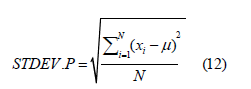
where: x_i = each number in the population, N = total number of numbers in the population and , is the population mean.

Fgure 5:Temporal water elevation across three different grid resolutions.

The computed population standard deviations between the three model resolutions, 0.24m at Monitor 1, 0.22m at Monitor 6 and 0.24m at Monitor 9, describe the magnitude of variability associated with the different spatial resolutions.

ERA5 data

Atmospheric forcing was derived from the ERA5 reanalysis dataset, produced by the European Centre for Medium-Range Weather Forecasts (ECMWF). ERA5 provides hourly global atmospheric fields at high spatial resolution and is widely used in hydrodynamic and flood modeling due to its reliability and temporal continuity [26]. A Python processing script was implemented to extract and convert key meteorological variables into Delft3Dcompatible formats. The following parameters were retrieved from the NetCDF file: 10-m zonal and meridional wind components (u10, v10), mean sea-level pressure (msl) and surface pressure (sp) converted from pascals to millibars, total cloud cover (tcc), and 2-m air and dew-point temperatures (t2m, d2m) converted from Kelvin to degrees Celsius. Additional hydrometeorological fields included the accumulated shortwave downward radiation (avg_snswrf) and total precipitation (tp) converted from meters to millimeters. Rainfall intensity was derived from the precipitation rate (avg_tprate) and expressed in mm/h. All values were read using the CF-compliant metadata contained in the file header, ensuring consistency with the ERA5 GRIB-to-NetCDF conversion conventions. These processed variables were subsequently used as spatially and temporally varying boundary conditions in Delft3DFLOW.

Delft3D’s performance metrics

To evaluate the performance of the Delft3D-FLOW simulations, modeled results were compared against observed flow velocities, water levels and inundation extents derived from field measurements and remote sensing data. Two primary performance metrics were employed to quantify model accuracy and spatial agreement. The first metric is widely used in hydrodynamic and flood modeling studies [27], while the second metric has recently been applied in environmental transport and hazard modeling [28,29].

(a) Success Rate (SR): The SR quantifies the spatial overlap between the model-predicted inundated area and the observed flood extent. It is defined as:

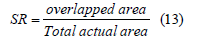
where: the Overlapped area represents the intersection between the modeled inundation and the observed flood extent, and the Total observed area is the flood area measured in situ or via satellite imagery. The SR ranges from 0 (no overlap) to 1 (perfect agreement). Note that SR does not penalize predicted flooded areas outside the observed extent.

(b) Failure Rate (FR): The FR is a measure used to quantify how much of the modelled flooded area falls outside the observed extent.

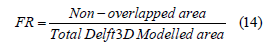
where: The non-overlapped area corresponds to the portion of the modelled flooded area that does not intersect with the observed (SAR-derived) flooded extent. The total modelled flooded area represents the full flooded extent produced by the models. FR ranges from 0 in the best case, when the entire modelled flooded area lies within the observed flooded extent, to 1 in the worst case, when the modelled flooded area does not overlap the observed extent at all.

(c) Centroid Skill Score (CSS): The CSS evaluates how closely the centroid of the modeled inundation matches the observed centroid, providing a measure of spatial accuracy. First, the Centroid Displacement Index (CI) is calculated as:

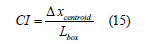
where: Δ_xcentroid is the distance between the geometric centers of the modeled and observed flooded areas, and L_box is the diagonal length of the bounding box enclosing the observed inundation.

The CSS is then defined as:

where: C_thr is a user-defined threshold specifying the acceptable centroid displacement. In this study, C_thr=1, meaning that the model is considered accurate if the centroid of the predicted flood remains within the characteristic length scale of the observed inundation.

This section presents the methodology used to simulate the hydrodynamics and flood propagation of the Pinios River during Storm Daniel. Following grid generation, the required boundary conditions were assigned to the Delft3D-FLOW model, including upstream river inflow hydrographs, tidal forcing at the estuarine outlet and spatially distributed rainfall and wind fields. Atmospheric forcing was derived from ERA5 reanalysis data, ensuring realistic representation of precipitation, evaporation and wind-driven effects throughout the domain. Accurate formatting and spatial alignment of these inputs were essential to maintain physical consistency and numerical stability during simulation. A detailed description of the hydrodynamic setup, bathymetric processing, boundary condition implementation and model validation is provided to outline the full simulation workflow applied in this study.

Delft3D-FLOW setup

(a) Domain: The hydrodynamic simulation of the Pinios River was performed using the Delft3D-FLOW module, operating in three-dimensional baroclinic mode to resolve vertical stratification and shear. The computational domain covered the full extent of the river, its floodplain, and the estuarine outlet at the Aegean Sea. The model was discretized on a rectangular Cartesian grid consisting of 712 points in the M-direction and 643 points in the N-direction, providing sufficient resolution to capture narrow channel sections, floodplain depressions, and tidal influence near the coast. Vertically, the water column was divided into 10 σ-layers with non-uniform thickness percentages, as described in Section 2.3.

(b) Time frame: The simulation was conducted over the period from 01 September 2023 00:00 UTC to 30 September 2023 00:00 UTC (~30days). The computational time step was set at 1 sec, selected based on a Courant–Friedrichs–Lewy (CFL) condition analysis to ensure numerical stability of the hydrodynamic solver. The CFL condition [6], defined as:

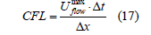
where: U_flow^max = the maximum flow velocity, Δt = the time step and Δx = the spatial resolution, was maintained below the stability threshold, typically less than 1 for explicit schemes. Considering the grid resolution (30m), time step (1s) and expected maximum flow velocities in the Pinios River (~5.0 m/s) [25], the resulting Courant number remained within the recommended safe range (CFL ≤ 0.33) across the entire model domain, ensuring numerical stability and accurate propagation of the flood wave.

(c) Boundary conditions: Meteorological forcing was obtained from the ERA5 reanalysis dataset [26], which provides hourly, spatially varying atmospheric fields on a global grid. The extracted variables included 10m wind components, mean sea-level and surface pressure, air temperature, dew-point temperature, cloud cover, shortwave radiation and precipitation. Wind forcing was applied to the hydrodynamic model in the form of shear stress acting on the free surface [6]. The wind shear stresses in the x- and y-directions (τ_sx, τ_sy) were computed as:

where: ρ_α = air density (1.1kg/m³), U_10m = wind speed at 10m height and θ = wind direction relative to the model grid axes, both derived directly from ERA5 outputs.

The stresses were converted into surface body forces F_x^wind and F_y ^wind acting on the upper water layer through:

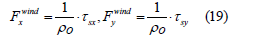
where: ρ_ο = 1026.72kg/m³, representing water density. The drag coefficient Cd was calculated using the piecewise formulation of Smith and Banke [6]:

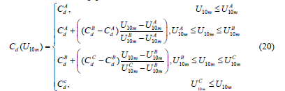
where: C_dⁱ = wind drag coefficients at the windspeed U_10mⁱ (i = A, B, C) and were selected based on literature values and verified against the fetch-limited wave conditions [30]. The values are shown in Table 1.

Table 1:Quantities of materials used.

Bottom friction in Delft3D-FLOW was parameterized with the Chezy formulation. A uniform Chezy coefficient C = 65 was adopted as a starting value, representing moderate bed roughness typical of mixed sediment and exposed rock channels. For a hydraulic radius of approximately 10m this Chezy corresponds to a Manning n on the order of 0.023, consistent with values reported for natural channels of similar character [31]. The Chezy formulation expresses bed shear stress τ_b as:

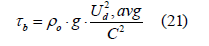
where: U_d,avg = depth-averaged velocity.

Lateral (wall) roughness was set to free-slip (wall roughness=0), assuming minimal resistance from the lateral boundaries such as vertical walls or embankments.

The downstream boundary at the Aegean Sea (Figure 6) was represented using a Riemann-type open boundary, which allows outgoing waves to propagate freely while accommodating incoming tidal forcing. Astronomical tidal constituents were prescribed as the primary forcing mechanism. The vertical distribution of velocities was defined using a logarithmic profile to better represent near-bed shear and the vertical structure of the flow. The M2 tidal constituent was imposed with an amplitude of 0.15m/s at a phase angle of 205°, while the S2 constituent was set to 0.07m/s with a phase of 220° [32]. These conditions provide realistic representation of tidal dynamics at the river mouth, ensuring accurate simulation of estuarine hydrodynamics and flood propagation in the lower Pinios River.

Fgure 6:Representation of the downstream open boundary at the Aegean Sea, showing the Riemann-type boundary.

(d) Turbulence and mixing processes: To simulate turbulent mixing in the Pinios River, the hydrodynamic model utilized the standard k-ε turbulence closure scheme, which is well-suited for stratified and shear-dominated flows in rivers and estuarine systems. Background (minimum) eddy viscosity and diffusivity values were prescribed to represent sub-grid mixing and maintain numerical stability in regions of weak turbulence:
A. Horizontal eddy viscosity: 0.02m²/s
B. Horizontal diffusivity: 0.002m²/s
C. Vertical eddy viscosity: 2 × 10-5m²/s
D. Vertical diffusivity: 2 × 10-4m²/s

These parameters fall within typical ranges for large riverine and estuarine environments, enabling the model to realistically capture vertical shear, stratification and mixing processes while limiting artificial numerical diffusion [6].

(e) Heat flux model: Surface heat exchange in the Pinios River and estuarine domain was simulated using Delft3D-FLOW’s heat flux module, which accounts for all major components of the surface energy budget, including incoming solar radiation, longwave radiation, sensible heat and latent heat fluxes. Shortwave radiation attenuation within the water column was parameterized using a Secchi depth of 5m, representing typical water clarity in the study area and controlling vertical penetration of solar energy.

Latent heat flux due to evaporation was computed using the Dalton formula, with a Dalton number of 0.0013, while convective heat exchange was governed by the Stanton number, also set to 0.0013. These values are representative of moderately turbulent atmospheric conditions over riverine and estuarine waters [6].

Meteorological forcing, air temperature, relative humidity, wind, and cloud cover was provided dynamically by ERA5 reanalysis data, ensuring temporal and spatial consistency between atmospheric conditions and the hydrodynamic model.
(f)Inflow discharge: The methodology for the hydrodynamic simulations involved prescribing an initial upstream inflow at Delft3D coordinates M73, N692 of approximately 10m³/s, consistent with literature values and representative of typical seasonal baseflow conditions for the Pinios River [25,33].

Python integration for simulation setup

Within the Delft3D interface, users can configure spatially and temporally varying wind and pressure conditions to drive hydrodynamic and meteorological simulations. The interface provides a comprehensive environment for defining physical, numerical, and operational parameters relevant to a wide range of environmental modeling applications..

On Figure7, ERA5-derived atmospheric forcing is highlighted. In the Wind tab under Physical Parameters, users can select wind and pressure fields that vary spatially or remain uniform. These fields are sourced from ERA5 reanalysis data, allowing the simulations to incorporate realistic, high-resolution historical weather conditions. On the right panel, the Additional Parameters section details the mapping of ERA5 variables (e.g., u10, v10, t2m, mslpressure) to internal Delft3D keywords such as Filwu and Filwt. This structure enables Python scripts to parse the ERA5 outputs and dynamically populate the required input files for each simulation run.

Fgure 7:Delft3D interface for adding ERA5 parameters.

The Python script developed for this study, create_ERA5_ parameters.py, is being released on GitHub to streamline this workflow. It generates ERA5-based input files for Delft3D, including:
a) u10 and v10: 10-meter wind components (m/s), defining wind speed and direction,
b) t2m and d2m: 2-meter air temperature and dew point temperature (°C),
c) mslpressure and surfpressure: mean sea level and surface pressures (mbar),
d) tcc: total cloud cover (%),
e) avg_snswrf: shortwave radiation flux (W/m²),
f) tp: total precipitation (mm),
g) avg_tprate: precipitation rate (mm/h).

These files are formatted for direct use in Delft3D, ensuring consistency between atmospheric forcing and hydrodynamic simulations.

Preparation of flood extent layers for model validation

The flood extent simulated by the Delft3D-FLOW model was compared against the observed inundation derived from the Copernicus Emergency Management Service (EMS) [34]. To ensure consistency between the two datasets, a structured geospatial workflow was implemented to preprocess and align their spatial representations. The objective of this workflow was to extract clean and directly comparable flood polygons from both the model results and the EMS dataset, enabling reliable computation of the validation metrics. Additionally, both datasets correspond to the same temporal reference, 10/09/2023 at 10:00 a.m., ensuring full alignment in terms of observation and simulation timing.

From the Delft3D simulation, the maximum inundation outline was exported as a shapefile in the coordinate reference system EPSG:32634 (WGS 84 / UTM zone 34N). This initial output included both overbanks flooded areas and the permanently wet river channel. Because the validation focuses exclusively on spillover processes and inland flood extent, the active river channel was manually removed in QGIS using standard vector editing tools. This resulted in two refined model-derived shapefiles describing the inundated areas north and south of the Pinios River, representing only the floodplain regions that were affected during the Daniel event.

The EMS flood (EMSR692) extent was provided as several vector tiles covering different parts of the study area. These tiles were first merged into a single shapefile and reprojected to EPSG:32634 to match the model’s spatial framework. To ensure spatial consistency, the merged EMS layer was clipped to the boundaries of the Delft3D computational grid. Subsequently, the northern and southern model flood polygons were used to clip the EMS dataset, producing two EMS-derived layers that match the exact spatial footprint of the corresponding model outputs. All geospatial operations, including merging, reprojection, and clipping, were automated using Python’s GeoPandas and Shapely libraries, ensuring reproducibility and consistent preprocessing across all datasets.

Section 4 presents the results of the study, beginning with the outcomes of the hydrodynamic modeling to simulate flood behavior. It then compares the modeled flood extents with data from the Emergency Management Services (EMS), providing an assessment of model accuracy and highlighting areas of agreement and discrepancy.

Hydrodynamic model results

Fgure 8:Average precipitation rate and inflow–outflow discharge variation during the Pinios River flood simulation..

The temporal evolution of the average precipitation rate (mm/h), derived from nine monitoring points across the Pinios River basin, along with the inflow and outflow discharges (m³/s), is presented in Figure 8 at the upstream inflow (Monitor 1) and downstream outflow (Monitor 9), respectively, as obtained from the Delft3D-FLOW simulation of the September 2023 “Daniel” flood event. The mean precipitation intensity ranged from 0 to 49mm/h, with the most intense rainfall occurring between simulation hours 78-153, corresponding to the peak of the storm system [12]. This rainfall led to a rapid increase in upstream inflow discharge (Monitor 1), rising from approximately 10m³/s at the onset [25,33] to a peak near 70m³/s, reflecting strong runoff generation and watershed response. The downstream outflow (Monitor 9) followed with a temporal lag of roughly 3-4 hours, peaking around 45-50m³/s. The discrepancy between inflow and outflow hydrographs indicates temporary water storage and attenuation within the river reach, consistent with overbank inundation and floodplain retention processes simulated in Delft3D-FLOW. Overall, the combined precipitation and discharge patterns highlight the dynamic coupling between atmospheric forcing and hydrodynamic response in the Pinios River system under extreme meteorological conditions.

Figure 9 shows the reconstructed time-series profile of the Daniel flood system, that reveals a clear transition from an initial low-activity regime to a sustained period of elevated hydraulic response associated with the onset of flooding. Early values remain close to zero, indicating minimal system pressurization prior to the first measurable inflow at Monitor 1. Following this quiescent phase, the signal rises sharply toward approximately 0.6, marking the first pronounced inflow event and signaling the start of the flood, initiating a sequence of increasingly coherent oscillatory patterns. As the series progresses, both amplitude and variance increase, reflecting progressive system activation and the establishment of a stable inflow–outflow cycle characteristic of a flooding river network. Mid-sequence values commonly fluctuate between 1.0 and 1.8, suggesting that once the floodwaters begin to dominate, the system maintains a relatively high and consistent throughput. The later segments of the series exhibit the highest peaks, frequently exceeding 2.0, indicating intermittent surges during which outflow at Monitor 9 surpasses prior maxima, consistent with transient flood pulses or elevated downstream conveyance efficiency. This gradual escalation, followed by stabilized high-level oscillations, is characteristic of a system in which flood inflow pulses propagate and amplify through the hydraulic network until a dynamic equilibrium between Monitor 1 inflow and Monitor 9 outflow is established. Overall, the trajectory of the dataset portrays a controlled yet increasingly responsive hydrodynamic environment, where transient inflow drivers produce quantifiable and temporally structured flood behavior. The signal represents water elevation in meters, and the values reflect the temporal evolution of water levels across the nine monitoring points.

Fgure 9:Temporal water elevation at nine monitoring points and their average.

Flood extent comparison with EMS data

Figure 10 illustrates the flooding of the upstream (northern and western) banks of the Pinios River during the Daniel event. The DELFT3D–EMS comparison (Appendix 1) demonstrates strong consistency in inundation mapping, supported by the high SR value (0.941) and the low FR (0.096). The CI of 0.012 indicates minimal spatial disagreement between the datasets, while the CSS of 0.988 confirms that the model accurately identifies true flooded areas with very few false classifications. Elevation comparisons reinforce these findings: lower EMS elevation classes (0.15-0.50m) correspond well with DELFT3D’s 0.25–0.75m range, and mid-range EMS elevations (1.00-2.00m) consistently match with 1.50-2.00m in the model. Although EMS high-elevation areas (4.00-6.00m) align with a slightly lower DELFT3D band (2.00-2.75m), the overall spatial distribution remains coherent (Appendix 2). These patterns indicate that DELFT3D captures the upstream flood behaviour effectively, with minor vertical underestimation that does not substantially affect the representation of inundation extent.

Fgure 10:Upstream Flooded Banks (Northern and Western River Banks).

Fgure 11:Downstream Flooded Banks (Southern and Eastern River Banks).

Figure 11 presents the downstream (southern and eastern) banks, where the alignment between DELFT3D and EMS is even stronger. The model achieves an SR of 0.947 and an FR of 0.069, while the exceptionally low CI (0.002) and the near-perfect CSS (0.998) indicate extremely high agreement in flood detection and spatial accuracy (Appendix 1). Elevation comparisons further highlight this performance: EMS values of 0.50-1.00m correspond tightly to the DELFT3D 0.75-1.00m class, and mid-elevation ranges of 2.00-4.00m align consistently with 2.00-3.00m in the model. Even for higher EMS elevations (4.00-6.00m), the DELFT3D range of 2.50-4.15m preserves the correct inundation pattern despite modest vertical compression (Appendix 2). These results suggest that the smoother topographic gradients and broader floodplain geometry of the downstream section enable DELFT3D to reproduce inundation characteristics with enhanced accuracy compared to the upstream segment.

Appendix 1::Comparison of DELFT3D vs EMS.

Appendix 2::Water elevation of DELFT3D vs EMS.

Section 5 presents a detailed discussion and assessment of the impacts observed, providing insight into the broader significance of the event. It begins by contextualizing the event and evaluating its overall importance, followed by an analysis of spatial patterns to understand how impacts are distributed across different areas. The section concludes with an exploration of the implications for public health and societal well-being, highlighting the relevance of the findings for both communities and policy-making.

Context and event significance

Flood impact assessment is a central element of flood risk management, as large-scale inundation influences not only hydraulic conditions but also environmental, socio-economic and public health systems. The Thessaly plain, one of Greece’s most important agricultural regions, is predisposed to flooding due to its broad, gently sloping terrain and extensive cultivation. Previous studies demonstrate that land-use patterns, slope variability, drainage density and soil characteristics strongly influence the spatial distribution of flood hazard in the basin, contributing to the severity of impacts during extreme events [35].

Storm Daniel, which struck Thessaly in September 2023, exemplified the magnitude of risk in this landscape. Remotesensing analyses revealed one of the most extensive inundation footprints recorded in the region, with floodwaters affecting agricultural land, transportation corridors and rural settlements at an unprecedented scale [36]. The validated alignment between the Delft3D-FLOW simulation and the Copernicus EMS observations, achieved through the geospatial workflow in Section 3.3, provides a reliable basis for interpreting these impacts. Ensuring consistency between simulated and observed flood extents is essential for identifying exposed areas, mapping critical zones and supporting informed decisions related to emergency response, spatial planning, and infrastructure protection.

Spatial patterns of impact

The validated flood extent reveals a distinct spatial distribution of impacts along the lower Pinios corridor, from the region of Larisa to the river’s outflow near Kouloura. North of Larisa, floodwaters dispersed across the wide agricultural plain, producing shallow but extensive inundation that corresponds closely with the EMS observations and the satellite-derived mapping of Daniel’s impacts [36]. This sector experienced considerable agricultural disruption and damage to rural transport links.

Further downstream, near Gonnoi, the flood formation changed markedly as the valley narrowed and the river’s meandering course constrained flow. This resulted in locally deeper and more concentrated inundation, a pattern consistent with findings from earlier hydrodynamic studies that describe the increased flood sensitivity of confined river reaches [37]. Eastward toward the estuary, floodwaters again spread laterally across low-lying terrain, affecting cultivated land and transportation infrastructure. Overall, the distribution of impacts in the modelled area reflects how the shape of the floodplain, the narrowing of the river channel, and local land uses influenced the flooding, and matches well with the damage patterns documented for the Daniel event.

Public health and societal relevance

The consequences of Storm Daniel extended beyond physical damage, influencing public health conditions across the affected communities. In the months following the event, health authorities recorded significant increases in waterborne and vector-borne diseases, including outbreaks of leptospirosis and gastrointestinal infections, as well as a marked rise in West Nile Virus incidence. The same period saw an estimated excess mortality of 335 deaths in the wider affected regions, highlighting the depth of the crisis and its sustained effect on societal resilience [38]. These outcomes underline the importance of accurate and timely flood extent mapping, as understanding inundation patterns is essential for anticipating health risks, guiding emergency response and strengthening preparedness strategies.

A couple of limitations affected the modelling and validation procedures and should be considered when interpreting the results. The modelling setup was developed under practical constraints regarding the availability of detailed bathymetric data for the Pinios River. Several reaches lacked full cross-sectional surveys and were completed through interpolation, a standard practice that provides geometric continuity. These constraints do not compromise the overall model integrity but should be considered when interpreting fine-scale water level variations within the domain.

The model employs a uniform Chezy coefficient (C=65) to represent bed friction. Although this value is consistent with Manning n ≈ 0.023 for typical hydraulic radii and falls within the range reported for natural mixed-sediment channels, it does not account for potential spatial variability in roughness across the floodplain or along the channel. Variations in vegetation, bank conditions and overbank flow resistance may influence local water depths and inundation extent. Due to the lack of detailed land-cover or field roughness measurements, spatially varying roughness could not be implemented in this study. This simplification should therefore be considered when interpreting the results and future work should incorporate spatially distributed or calibrated roughness fields when such data become available [39].

A second limitation relates to the temporal mismatch between the simulated peak inundation and the observational data available for validation. Analysis of the modelled water-level time series shows that maximum flooding occurred between 90 and 140 hours after 1 September, corresponding to 5-7 September 2023, when Storm Daniel delivered its most intense rainfall. In contrast, the Copernicus EMS flood delineation corresponds primarily to 10 September and after. By this time, floodwaters had already begun to recede across the lower Pinios corridor, leading to observed flood extents that reflect a post-peak rather than peak-inundation condition. Consequently, the EMS polygons cannot fully represent the maximum spatial footprint of the event. These factors should be taken into account when interpreting spatial discrepancies within the modelled domain, particularly in areas where flood recession was rapid following the end of the storm.

This study demonstrates that a high-resolution Delft3D-FLOW model, driven by ERA5 atmospheric reanalysis, can successfully reconstruct the flood dynamics associated with Storm Daniel along the Pinios River. By integrating a 3D σ-coordinate grid with available bathymetry and a reproducible Python-based preprocessing workflow, the modelling framework captures the hydrodynamic response to the extreme rainfall of early September 2023 and reproduces the primary inundation patterns observed in the field. The validated flood extent reflects the transition from confined valley reaches to broader floodplain areas in northeastern Thessaly, in strong agreement with Copernicus EMS mapping.

The work highlights the value of combining hydrodynamic modelling with geospatial alignment techniques to obtain reliable flood extent evaluations in data-limited environments. The structured workflow for harmonizing model outputs with EMS observations proved critical for ensuring spatial consistency and deriving robust performance metrics. These findings underscore the broader potential of Delft3D-FLOW, coupled with atmospheric reanalysis datasets, to support flood risk assessment, emergency planning and resilience-oriented decision-making.

Although constrained by incomplete bathymetric data and a temporal mismatch between modelled peak inundation and available EMS observations, the study demonstrates that meaningful validation is achievable through careful interpretation. Future research should incorporate higher-resolution channel geometry, time-synchronous satellite products, and coupled hydrometeorological simulations to improve peak-flood representation. Overall, the framework provides a transferable modelling– validation approach that can be applied to other flood-prone basins facing similar data limitations.

This work was supported by ECHO/G.A. 101225575/HE LUMP SUM.

V.P. conceived the study and wrote the abstract; V.P. and D.V. wrote the introduction and results; V.P. prepared the ERA5 data implementation; D.V. and C.A. prepared the figure illustrations; A.M. reviewed the first draft; A.M. and I.G. supervised the methodology and conclusions sections; S.V. and I.K. acquired the funding. All authors have read and agreed to the published version of the manuscript.

The authors declare no conflict of interest.

ERA5 input data and the generated Delft3D-compatible output files used in this study are publicly available. The Python scripts developed to process and convert ERA5 meteorological fields into the required Delft3D input format can be accessed at https:// github.com/vaspapa79/Delft3D_ERA5.git

1. Guyasa AK, Zhang D, Guan Y, Niyongabo A, Ziyuan W, et al. (2025) Climate change impacts on river flow and extreme hydrological events in the Tendaho Catchment, Ethiopia. Journal of Water and Climate Change 16(11): 3243-3274.
2. Kundzewicz ZW, Lugeri N, Dankers R, Hirabayashi Y, Döll P, et al. (2010) Assessing river flood risk and adaptation in Europe-Review of projections for the future. Mitigation and Adaptation Strategies for Global Change 15(7): 641-656.
3. Wu Y, Ju H, Qi P, Li Z, Zhang G, et al. (2023) Increasing flood risk under climate change and social development in the second Songhua river basin in Northeast China. Journal of Hydrology: Regional Studies 48: 101459.
4. Sanders BF (2017) Hydrodynamic modeling of urban flood flows and disaster risk reduction. Oxford University Press.
5. Mahmood MQ, Wang X, Aziz F, Dogulu N (2025) Urban flood modelling: Challenges and opportunities-A stakeholder informed analysis. Environmental Modelling & Software 191: 106507.
6. Delft Hydraulics (2024) User manual of Delft3D-FLOW: Simulation and multi-dimensional hydrodynamic flows and transport phenomena, including sediments. WL/Delft Hydraulics.
7. Mardani N (2021) Advances in hydrodynamic modelling of flow in rivers and estuaries using Lagrangian drifter data (Doctoral dissertation, University of the Sunshine Coast, Queensland).
8. Zellou O, Rahali H (2019) Assessment of the joint impact of extreme rainfall and storm surge on the risk of flooding in a coastal area. Journal of Hydrology 569: 647-665.
9. Kuntinah K, Nugraheni I, Ardianto R (2021) The simulation of water level using Delft3D hydrodynamic model to analyze the case of coastal inundation in Pontianak. Innovative Technology and Management Journal 4(1): 32-44.
10. Kerin I, Giri S, Bekic D (2018) Simulation of levee breach using Delft models: A case study of the Drava River flood event. In Flood risk assessment and management, pp. 1117-1131.
11. Vanden Bout B, Jetten VG, Van Westen CJ, Lombardo L (2023) A breakthrough in fast flood simulation. Environmental Modelling & Software 168: 105787.
12. Lekkas E, Diakakis M, Mavroulis S, Filis C, Bantekas I, et al. (2024) The early September 2023 Daniel storm in Thessaly Region (Central Greece).
13. He K, Yang Q, Shen X, Dimitriou E, Mentzafou A, et al. (2024) Brief communication: Storm Daniel flood impact in Greece in 2023: Mapping crop and livestock exposure from synthetic-aperture radar (SAR). Natural Hazards and Earth System Sciences 24(7): 2375-2382.
14. Psomas A, Dagalaki V, Panagopoulos Y, Konsta D, Mimikou M (2016) Sustainable agricultural water management in Pinios River Basin using remote sensing and hydrologic modeling. Procedia Engineering 162: 277-283.
15. Fytianos K, Siumka A, Zachariadis GA, Beltsios S (2002) Assessment of the quality characteristics of Pinios River, Greece. Water, Air & Soil Pollution 136: 317-329.
16. Stefanidis K, Panagopoulos Y, Psomas A, Mimikou M (2016) Assessment of the natural flow regime in a Mediterranean river impacted from irrigated agriculture. Science of the Total Environment 573: 1492-1502.
17. Billen G, Garnier J (2007) River basin nutrient delivery to the coastal sea: Assessing its potential to sustain new production of non-siliceous algae. Marine Chemistry 106(1-2): 148-160.
18. Loukas A, Mylopoulos N, Vasiliades L (2007) A modeling system for the evaluation of water resources management strategies in Thessaly, Greece. Water Resources Management 21(11): 1673-1702.
19. Stamatis G, Parpodis K, Filintas A, Zagana E (2011) Groundwater quality, nitrate pollution and irrigation environmental management in the Neogene sediments of an agricultural region in central Thessaly (Greece). Environmental Earth Sciences 64(4): 1081-1105.
20. Burchard H (2001) Simulating the wave-enhanced layer under breaking surface waves with two-equation turbulence models. Journal of Physical Oceanography 31(11): 3133-3145.
21. Papaioannou V, Mantsis DF, Anagnostopoulos CGE, Vlachos K, Moumtzidou A, et al. (2025a) Integrated hydrodynamic and atmospheric modeling of Polyfytos Lake for substance dispersion using Delft3D and weather research and forecasting model. Open Journal of Civil Engineering 15(2): 223-248.
22. Papaioannou G, Vasiliades L, Loukas A, Alamanos A, Efstratiadis A, et al. (2021) A flood inundation modeling approach for urban and rural areas in lake and large-scale river basins. Water 13(9): 1264.
23. Papagiannaki K, Kotroni V, Lagouvardos K, Koutroulis AG, Michaelides S (2025) Rainfall patterns and their association with flood fatalities across diverse Euro-Mediterranean regions over 41 years. NPJ Natural Hazards 2: 39.
24. Xie Q, Liu Z, Fang X, Chen Y, Li C, et al. (2017) Understanding the temperature variations and thermal structure of a subtropical deep river-run reservoir before and after impoundment. Water 9(8): 603.
25. Koutras A (2024) Statistical analysis of river environmental data. (Master’s thesis, University of Thessaly, Department of Agriculture, Ichthyology and Aquatic Environment). University of Thessaly Institutional Repository, p. 30641.
26. Hersbach H, Bell B, Berrisford P, Hirahara S, Horányi A, et al. (2020) The ERA5 global reanalysis. Quarterly Journal of the Royal Meteorological Society 146(730): 1999-2049.
27. Wing OEJ, Bates PD, Sampson CC, Smith AM, Johnson KA, et al. (2017) Validation of a 30m resolution flood hazard model of the conterminous United States. Water Resources Research 53(9): 7968-7986.
28. Papaioannou V, Anagnostopoulos CGE, Moumtzidou A, Gialampoukidis I, Vrochidis S, et al. (2025b) Application of OpenOil in modeling a shipwreck oil spill: The Tobago case. Computational Water, Energy, and Environmental Engineering 14(4): 151-177.
29. Dearden C, Culmer T, Brooke R (2022). Performance measures for validation of oil spill dispersion models based on satellite and coastal data. IEEE Journal of Oceanic Engineering, 47(1): 126-140.
30. Lin W, Sanford L, Suttles S, Valigura R (2002) Drag coefficients with fetch-limited wind waves. Journal of Physical Oceanography 32: 3058-3074.
31. Hsu YL, Dykes JD, Allard RA, Kaihatu JM (2006) Evaluation of Delft3D performance in nearshore flows (NRL/MR/7320–06 8984). Naval Research Laboratory, Oceanography Division.
32. Arabelos D, Papazachariou D, Contadakis M, Spatalas S (2011) A new tide model for the Mediterranean Sea based on altimetry and tide gauge assimilation. Ocean Science 7(3): 429-437.
33. Panagopoulos Y, Makropoulos C, Gkiokas A, Kossida M, Evangelou E, et al. (2014) Assessing the cost-effectiveness of irrigation water management practices in water stressed agricultural catchments: The case of Pinios. Agricultural Water Management 139: 31-42.
34. Copernicus Emergency Management Service (2023) Rapid mapping activation EMSR692 – Flood in Greece (Storm Daniel, September 2023). Vector products: EMSR692_AOI03_DEL_PRODUCT_waterDepthA_v3 and EMSR692_AOI04_DEL_PRODUCT_waterDepthA_v2.
35. Alafostergios N, Evelpidou N, Spyrou E (2025) Flood susceptibility assessment based on the analytical hierarchy process (AHP) and geographic information systems (GIS): A case study of the broader area of Megala Kalyvia, Thessaly, Greece. Information 16(8): 671.
36. Falaras T, Dosiou A, Tounta S, Diakakis M, Lekkas E, Parcharidis I (2025) Mapping of flood impacts caused by the September 2023 Storm Daniel in Thessaly’s Plain (Greece) with the use of remote sensing satellite data. Remote Sensing 17(10): 1750.
37. Oikonomou A, Dimitriadis P, Koukouvinos A, Tegos A, Pagana V, et al. (2013) Floodplain mapping via 1D and quasi-2D numerical models in the valley of Thessaly, Greece. In European Geosciences Union General Assembly 2013, Geophysical Research Abstracts (Vol. 15, EGU2013-10366). European Geosciences Union.
38. Kondilis E, Valavani E, Bellos V, Benos A (2025) Floods and public health: The impacts of Storm Daniel on the health of the population in Thessaly and Central Greece. ΚΕΠΥ Policy Report 2025.1.
39. Stefanyshyn D, Khodnevych Y, Korbutiak V (2021) Estimating the Chézy roughness coefficient as a characteristic of hydraulic resistance to flow in river channels: A general overview, existing challenges, and ways of their overcoming. Environmental Safety and Natural Resources 39(3): 16-43.