
- About Us
- Information
-

The Author ensures that the research has been conducted responsibly and ethically with adherence to all relevant regulations. read more..
- For Authors
- For Reviewer
- Manuscript Guidelines
- Membership
- Publication Ethics
-
- Journals
- Reprints
- e-Books
- Videos
- Policies
- Contact Us
 COVID-19
- Submissions


Full Text
Advancements in Civil Engineering & Technology
Analytical Solutions of a Conduction Problem with Two Different Kinds of Boundary Conditions
Zhongzhi Fu2*, Qiming Zhong1 and Shengshui Chen2
1 Department Geotechnical Engineering, Nanjing Hydraulic Research Institute, China
2 Key Laboratory of Failure Mechanism and Safety Control Techniques of Earth-Rock Dams, Ministry of Water Resource, China
*Corresponding author: Zhongzhi Fu, Key Laboratory of Failure Mechanism and Safety Control Techniques of Earth-Rock Dams, Ministry of Water Resource, China
Submission: May 30, 2018;Published: August 28, 2018

ISSN 2639-0574Volume2 Issue2
Abstract
A heat transfer problem was taken as an example to provide the analytical solutions of a one-dimensional conduction problem with two different kinds of boundary conditions. The theoretical solutions were obtained by using the method of separation of variables for solving partial differential equations. Temperature distribution in two simple cases were studied using the analytical solutions and were compared with corresponding numerical results. Reliability of the analytical results were shown by their excellent agreement with those numerical ones. The solutions presented in this note can be used for the verification of new numerical algorithms.
Keywords:Heat transfer; Conduction problem; Analytical solution; Boundary condition
Introduction
Conduction problems are widely encountered in science and engineering, such as heat transfer through conductive materials [1] and water flow through porous media [2]. Such physical processes are governed by similar differential equations and are studied traditionally by seeking the mathematical solutions. However, analytical solutions can only be derived under very limited simple boundary and initial conditions [3]. Therefore, much efforts have been spent in developing numerical tools since the popularization of computers [4], and the finite element method (FEM) is, probably, the most successful and widely used one [5]. Use of the FEM usually needs the discretization of both the space and the time, and a more refined mesh and a smaller time step generally yield more exact numerical results. However, this is not the case for conduction problems as unreasonable oscillatory results are often obtained for a given mesh if the time step is smaller than a threshold value [6-9]. For instance, use of four-noded rectangular elements for conduction problems without causing oscillatory results needs the time increment (Δt) larger than L2c/(2k), while for eight-noded elements the threshold is reduced to L2c/(20k). Herein, L denotes the characteristic length of elements while c and k are volumetric capacity and conductivity coefficient of the concerned material [7]. The dilemma, on the other hand, is that a small enough time step is required for numerical convergence for problems where nonlinear material behavior presents [8-10]. It was found that the traditional mass-distributing scheme, which yields the so-called consistent mass matrix, may generate an incorrect neighboring nodal response even though the physical laws are correctly applied at the elementary level. Pan et al. [9] therefore suggested two new mass-distributing schemes which were free of numerical oscillation. Alternatively, mass lumping techniques yielding a diagonal mass matrix were employed by many other authors to remove the possible numerical oscillation [11-13]. Some special techniques were also proposed in the framework of finite element method (known as the stabilized finite element methods) to repress the unphysical oscillations, as recently reviewed and compared by Sendur [14].
No matter what kind of mass matrix or numerical strategy is used, an indispensable step of developing a numerical scheme is the verification of the obtained results for some benchmark problems against the correct ones, and a closed-form solution is unquestionably the best reference for this purpose. In this short note, analytical solutions of a conduction problem with two specific boundary and initial conditions were provided and compared with the corresponding numerical results. The problem and analytical solutions can be used as basic benchmark cases in verifying numerical schemes for conduction problems.
Problem definition
Let us take the heat transfer problem in Figure 1 as an example. The lower boundary (z=0) of an infinite layer of conductive material is exposed to some temperature change or heat flux, and the problem is to find out the temperature distribution within the conductive material. In this note, we assume that all the thermal variables at a horizontal plane are the same. So, the temperature varies only vertically, and this problem is in fact one-dimensional.
Figure 1:Definition of the one-dimensional heat transfer problem.

According to Fourier’s law of heat conduction [1], the heat flux through a horizontal plane, denoted by q, is negatively proportional to the temperature gradient as follows:
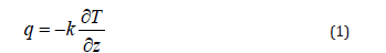
in which T is the temperature and k denotes the thermal conductivity. The net heat entering the differential layer (dz) of material results in an increase of the temperature, i.e.
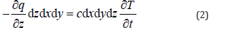
in which c denotes the volumetric heat capacity of the material, and the lowercase t stands for the time. Inserting Equation (1) into Equation (2) and neglecting the spatial variation of the thermal conductivity, one obtains the following governing equation for the one-dimensional heat transfer problem:
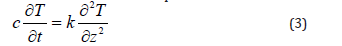
Similar form of equations can also be obtained for other conduction problems.
The upper boundary (z=H) of the material layer is assumed adiabatic and heat can only flow from the lower boundary (z=0). Two kinds of boundary conditions were considered herein. Firstly, the temperature at the lower boundary was increased linearly from T0 to T1 during the period of 0~t1, as shown in Figure 1. Secondly, a constant heat flux, q0, was input from the lower boundary to the conductive layer, as shown in Figure 1. In both cases, the initial temperature was assumed homogeneous within the material, i.e. T (t=0) =T0.
Analytical solutions
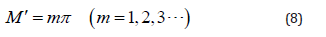
For both boundary conditions given above, Equation (3) can be solved using the standard method of separation of variables [15]. In this part, only the analytical results were given. The solution for the temperature boundary problem (Figure 1) reads:
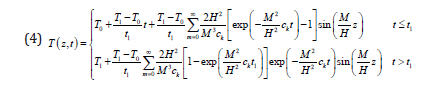
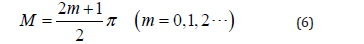
The analytical solution for the flux boundary problem described in Figure 1 reads:
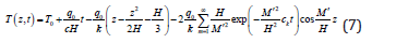
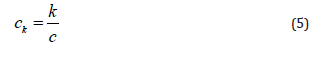
in which
The detailed derivation of the above solutions were not included in this short note. However, they were verified against numerical results in the next part.
Verification
In this part, two cases were studied to verify the analytical solutions. The temperature distribution obtained by Equation (4) and Equation (7) were compared with those predicted by a twodimensional finite element procedure [16]. The program was initially developed for unsaturated soil mechanical problems. However, the seepage module can also be used to study the conduction problem in a straightforward way.
Figure 2:The temperature distribution during boundary heating.

Case 1: The initial temperature within the conductive layer (H=1.0m) was 0 ℃, and the temperature at the lower boundary was increased to 10 ℃ in 120s. After the heating period (0~120s), the lower boundary temperature was kept constant. If the thermal conductivity of the material was k=1.0×10⁻⁹W/(m·K), and the volumetric heat capacity was c=1.0×10⁻⁵J/(m3·K), how will the temperature field evolve? Figure 2 and Figure 3 plot the temperature distribution during and after boundary heating, respectively. The curves plotted were the analytical solution given by Equation (4) and the black and bright circles and triangles were the results obtained by numerical simulation. Both 4-nodes quadrilateral elements and 8-nodes quadrilateral elements were used, and for both types of elements consistent mass and lumped mass were employed. Note that the diagonal mass matrices for 4-nodes elements were formed by summing all the entries in the same rows of the consistent mass matrices, and the lumped mass matrices for 8-nodes elements were formed according to the HRZ scheme [17]. The restrictions for time increment suggested by Thomas & Zhou [7] were used to guarantee non-oscillatory results when the consistent mass scheme was employed. It can be seen that all the numerical results coincide almost exactly with the analytical solution both during and after the boundary heating period, and the numerical and analytical results verify each other mutually. In addition, the results shown in Figure 2 and Figure 3 indicate that using mass-lumping schemes can also yield sufficiently reliable results with, however, no restriction on time steps.
Figure 3:The temperature distribution after boundary heating.

Case 2: The initial temperature within the conductive layer was again set to 0 ℃, and in this case a constant thermal flux of 1.0×10- 3W/m2 was input from the lower boundary to the conductive layer. The thermal conductivity and the volumetric heat capacity of the material were identical to those in case 1, i.e. k = 1.0×10- 9W/(m·K) and c=1.0×10⁻⁵J/(m3·K), how will the temperature field evolve? Figure 4 plots the numerical and analytical temperature distribution during heat flux inputting. Herein, both 4-nodes and 8-nodes quadrilateral elements with consistent mass and lumped mass were also used similarly. It is clear that the temperature near the lower boundary increases very rapidly in the current case. However, the variation of temperature near the upper boundary is much slower, agreeing well with an intuitive conjecture. The numerical results obtained in this case also coincide almost exactly with the analytical ones predicted by Equation (7), proving the reliability of the mathematical solution given above.
Figure 4:The temperature distribution during heat flux inputting.

Equation (4) and Equation (7) also provide some hints on the evolution of temperature field. For instance, Equation (4) states that the temperature distribution for the first case depends only on the ratio between the thermal conductivity and the volumetric heat capacity (ck=k/c) but is not influenced by the absolute values of both parameters. On the other hand, the volumetric heat capacity has a significant influence on the temperature evolution in the second case as indicted by Equation (7), i.e. a higher volumetric heat capacity results in a slower temperature increasing rate, and vice versa.
Conclusion
Conduction problems are difficult to solve by the finite element method in the sense that the time steps cannot be chosen arbitrarily. Precision and convergence of the results need the time steps to be small enough. But, unfavorable numerical oscillation may occur if the time steps were reduced to be smaller than certain threshold values. Different numerical schemes may be developed to conquer the dilemma. However, reliable results which can be used to verify these numerical schemes are scarce, even for those simplest onedimensional conduction problems. In this note, analytical solutions for a one-dimensional conduction problem with two kinds of boundary conditions were provided using the method of separation of variables. The solutions were expressed as sum of a series of sine and cosine functions, depending on the boundary conditions. The temperature distribution for two cases, one for a given temperature boundary and the other one for a given flux boundary, were studied using both the analytical solutions and corresponding finite element simulations. The numerical results and theoretical ones agree almost exactly with each other at different time instants in both cases, proving the correctness of the analytical solutions. Numerical results also show that using mass-lumping techniques, which were generally used to eliminate numerical oscillation, can also yield precise enough results. Analytical solutions given in this note can be used to verify new numerical schemes.
References
- Baehr HD, Stephan K (2011) Heat and mass transfer. (3rd edn), Springer, London.
- Fredlund DG, Rahardjo H (1993) Soil mechanics for unsaturated soils. John Wiley & Sons, Chichester, UK, p. 544.
- Kolditz O, Shao H, Wang W, Bauer S (2015) Thermo-hydro-mechanicalchemical processes in fractured porous media: modelling and benchmarking. Springer, London.
- Cheney W, Kincaid D (2008) Numerical Mathematics and Computing. (6th edn), Thomson Brooks/Cole, Belmont, USA.
- Zienkiewicz OC, Taylor RL, Zhu J Z (2013) The finite element method: its basis and fundamentals. (7th edn), Butterworth-Heinemann, London.
- Vermeer PA, Verruijt A (1981) An accuracy condition for consolidation by finite elements. International Journal for Numerical and Analytical Methods in Geomechanics 5(1): 1-14.
- Thomas HR, Zhou Z (1997) Minimum time-step size for diffusion problem in FEM analysis. International Journal for Numerical Methods in Engineering 40(20): 3865-3880.
- Karthikeyan M, Tan TS, Phoon KK (2001) Numerical oscillation in seepage analysis of unsaturated soils. Canadian Geotechnical Journal 38(3): 639-651.
- Pan L, Warrick AW, Wierenga PJ (1996) Finite element methods for modeling water flow in variably saturated porous media: Numerical oscillation and mass-distributed scheme. Water Resources Research 32(6): 1883-1889.
- Celia MA, Bouloutas ET, Zarba RLA (1990) General mass-conservative numerical solution for the unsaturated flow equation. Water Resources Research 26(7): 1483-1496.
- Ju SH, Kung KJS (1997) Mass types, element orders and solution schemes for the Richards’ equation. Computers and Geosciences 23(2): 175-187.
- Wu MX (2010) A finite-element algorithm for modeling variably saturated flows. Journal of Hydrology 394(3-4): 315-323.
- Vogel T, Genuchten MT, Cislerova M (2001) Effect of the shape of the soil hydraulic functions near saturation on variably-saturated flow predictions. Advances in Water Resources 24(2): 133-144.
- Sendur A (2018) A comparative study on stabilized finite element methods for the convection-diffusion-reaction problems. Journal of Applied Mathematics 2018: 1-16.
- Kreyszig E (2010) Advanced engineering mathematics. (10th edn), John Wiley & Sons, Jefferson City, Missouri, USA.
- Fu ZZ, Chen SS, Wei KM (2014) Unsaturated consolidation analysis program for earth and rockfill structures, theory and manual. Research Report of Nanjing Hydraulic Research Institute, Nanjing, China.
- Hinton E, Rock T, Zienkiewicz OC (1976) A note on mass lumping and related processes in the finite element method. Earthquake Engineering and Structural Dynamics 4(3): 245-249.
© 2018 Zhongzhi Fu. This is an open access article distributed under the terms of the Creative Commons Attribution License , which permits unrestricted use, distribution, and build upon your work non-commercially.
Editor In Chief


.jpg)


Signup for Newsletter

Quick Links
 Editorial Board Registrations
 Submit your Article
 Refer a Friend
 Advertise With Us
Our Recent Edition

.jpg)


Top Editors


.jpg)


.bmp)
.jpg)
.png)
.jpg)


.jpg)


.png)

.png)


.png)


Financial Support

Sponsors

Latest e-Books

Latest Video

 a Creative Commons Attribution 4.0 International License. Based on a work at www.crimsonpublishers.com.
Best viewed in
a Creative Commons Attribution 4.0 International License. Based on a work at www.crimsonpublishers.com.
Best viewed in