European Banking Efficiency: Economic Freedom and Camel Effects

After the recent financial crisis, European governments saw the need to launch a process of bank restructuring that incorporates a series of reforms based on country specific regulations. This process has evolved from a prudential regulation to a structural regulation which requires compliance with a set of rules, maintaining levels of asset quality and resources to address potential losses, provisioning for bad debts and compliance stress tests to ensure stability. The post-crisis situation in which these procedures have been developed has forced the governments to adopt new austerity measures and economic reforms that even nowadays continue to be implemented. Barth [1] explain that numerous pages of regulations in most countries delineate the permitted activities of banks and provide shape and substance to the deposit of insurance schemes and the nature and timing of the information that banks must disclose to regulators and the public. At the same time, numerous European governments have developed a climate of political instability which could be identified as cause and effect for all types of problems such as the appearance of corruption or the lack of transparency, among others [2]. In a context of bank restructuring of the European Union, where prudential measures have been implemented, based on specific regulations at both a domestic and European level, it is important to analyze how these new developments affect banks’ behavior, Michalak [3]; Elliot et al. [4]; Slimane et al. [5]; Milani [6] As the process of banking integration getting to conclude and such measures are being implemented progressively, it is interesting to evaluate banks’ efficiency and its variations during this restructuring. To this end, efficiency is estimated in a sample of 397 banks of 21 member states of the European Union in the period 2011-2014. The methodology used is nonparametric DEA for obtaining efficiency estimates. The aim of the second stage of the analysis is to identify which variables related with banks’ specific features and their states are determinants of their inefficiency levels. Specifically, the influence of the global management system CAMELS, the economic growth, and economic freedom variables are regressed on inefficiency by a regression model. Finally, the results show a significant influence of the global banks management system, CAMELS, as well as economic freedom variables in countries where they are located, on the levels of inefficiency of European banks analyzed during the period 2011-2014.

Review on banking efficiency

Efficiency is a key concept for financial institutions, and it has long been studied [7]. This is due to the recent events in the finance and banking environment, the study of evaluation and measurement of the efficiency of banks has given rise to a growing body of empirical literature [8]. The importance of the banking sector is premised on the grounds that banks are the main channels of savings and allocations of credit in an economy [9]. The banking sector provides important financial intermediation function by converting deposits into productive investments. Unlike in other developed nations where financial markets and the banking sector work in unison to channel funds, in developing countries, financial markets are undersized and sometimes completely absent [10]. It falls on the banking sector to bridge the gap between their efficiency in service delivery and their performance. According to the available literature, there are many researchers, who examine the efficiency of financial institutions by using methods such as parametric or non-parametric methods of banks Bopkin [7]; Alhassan 2016; Kablan [11].

Banking efficiency has often been analyzed in the European Union (EU). In this context, Fries [12] analyze efficiency in a sample of banks using efficiency as a proxy of progress associated with changes in structural and institutional reforms. Kasman [13] analyze efficiency in commercial banking in Central and Eastern European countries taking into account the impact of macroeconomic and financial sector conditions. Andries [14] show efficiency improvements may be due to increased competition upon EU accession and the entry of foreign banks. Chortareas [15] investigate the dynamics between bank regulatory and supervisory policies associated with EU banking efficiency from 2000 to 2006. Their evidence suggests that banks from countries with more open, competitive and democratic political systems are more likely to benefit from higher operating efficiency levels. Chortareas [16] study the relationship between financial freedom and commercial banks’ efficiency in EU. Tsionas [17] analyze efficiency in a sample of European banks in pre and post-crisis periods and demonstrate a decrease of efficiency after the crisis and an increase in the long term. On the other hand, the analysis of bank efficiency literature is central to the growth and long-term sustainability of the banking sector, especially in financial crisis period, Chen et al. [18]. There has been an abundance of research on the topic (Abreu et al. [19]; Aliyu et al. [20]; Bhatia et al. [21]; Lopes et al. [22].

Review on economic freedom

While the impact of economic freedom on the economy in general has been studied widely (see, for example, Adkins et al. [23]; Bergh [24]; Heckelman [25]) its impact on the Banking sector has only attracted the attention of researchers such as Claessens [26], Sufian [27], Chortaeas et al. [16] and Gropper et al. 2015, Bjornskov [28] and Asteriou et al. [29]. Chortaeas et al. [16]) indicate that excessive government interference in the activities of financial institutions, as reflected in the low scores of financial freedom rates, exercise a negative impact on bank efficiency. There are several reasons to think that economic freedom can have a positive impact on the behavior of bank sectors, improving their structure of results and the efficiency level. In their study, Claessens [26] point out that greater economic freedom by allowing new national and foreign participants to increase efficiency and allow a wider range of products that can improve banking gains. Economic freedom also means that banks tend to lend more, since there is likely more companies that compete in the economy and there will be a greater scope for banks to lend foreign companies and financial institutions that guarantee greater diversification in portfolios of bank loans and a return trade of higher risk of the banking system. It is also likely that greater economic freedom will lead to a better operational environment for business and stronger economic growth, resulting in a better banking performance measured by profitability and stability. In addition, countries with higher levels of economic freedom generally have higher levels of real income (Holmes et al. [30]), which in turn leads to a greater demand for banking services. They also argue that heavy banking regulation reduces opportunities and restricts economic freedom. In addition, Blau [31] argues that economic freedom reduces regulatory uncertainty, promotes free trade and these combined with greater emphasis on property rights reduce the probability of market accidents. This implies that economic freedom should be positive for both bank profitability and stability. A greater degree of economic freedom should generally lead to greater competition that can lead to lower inflation and a more stable macroeconomic environment. In his study, Chortaeas et al. [16] find that from 2000 greater economic freedom in 27 of the EU member states is associated with greater efficiency of the banking system. In a recent study, Asteriou et al [29] obtains that economic freedom has a positive effect on banking performance, obtaining a positive relationship between the levels of financial stability and the economic freedom of the country. Bjornskov [28] examines the impact of economic freedom on the risk of crisis and estimates the effects on duration, Pico to Regal GDP and the recovery times of 212 crisis in 175 countries during the period 1993-2010. The study suggests that economic freedom is strongly associated with smaller maximum relationships and a shorter recovery time. This implies that it will help increase profitability and bank stability. Economic freedom is also examined by Lin et al. [32] that focus on how financial freedom shapes the effect of changes in banking property in profitability. They find that a foreign presence facilitated by financial freedom improves bank efficiency. Since greater efficiency results in greater profitability and a lower risk of bankruptcy, then it implies that it improves the general performance of the banking sector.

Review on CAMELS model: Although a number of studies employ macroeconomic determinants to develop early warning systems for bank failures (Betz [33]; Mayes [34]; Rebel [35]), recent empirical evidence suggests that individual bank financial condition is a key driver in distinguishing their performance during the recent financial crisis (Berger [36]; Vazquez [37]). A large body of literature related to bank failure prediction focuses on the supervisory CAMELS indicator set. This is the acronym for capital, asset quality, management, earnings, liquidity, and sensitivity to market risk indicators, which are generally used by investors and regulators to assess the soundness of a financial institution. Several empirical studies also combine CAMELS with additional indicators (Cole [38], Altunbas 2011; Betz et al. [33]; Chiaramonte [39]. However, there is inconclusive evidence on which variables are important in predicting bank insolvencies. Poghosyan [40] show that indicators related to capitalization, assets and profitability can effectively identify weak banks. Berger [36] showed that capital had a positive impact on survival probabilities and market shares of small banks. While Mayes [41] indicated that leverage ratio outperforms weighted capital ratios on performance. In an attempt to receive a final answer as to which variables lead banks to default, this study incorporates a wide range of camel-related variables, along with various transformations, to identify those with the highquality power and provide a ranking among them. In this study, following the same philosophy, we use an extended dataset of bank-specific variables, testing their explanatory power, following the approaches used by (Mesai [42]; Cole [43]). The selection of variables is this research is in line with the ratios used in previous studies of bank behavior analysis. The C ratio was calculated as net capital among net loans (Wanke et al. [44]), the capital quality ratio, as deposits among total assets, while for the selection of the M variable, Roman [45] were followed. The E variable is measured as net income between average total assets (ROAA) (Wanke et al. [46]). The liquidity variable was obtained using loans over deposits (Rozzani [47]) and risk sensitivity using bank assets among total banking system assets (Roman [45]).

The DEA models

One of the most widely used methods in assessing the efficiency of a set of DMUs (Decision Making Units) is Data Envelopment Analysis (DEA). DEA is a non-parametric method which uses linear programming techniques to identify an efficiency frontier on which only the efficient Decision-Making Units (DMUs) are placed. First presented in 1978, and based on Farrell, the first DEA model is known in the literature as the CCR model, after its authors, Charnes, Cooper and Rhodes. Thus, by using linear programming and by applying nonparametric techniques of frontier estimation, the efficiency of a DMU can be measured by comparing it with an identified frontier of efficiency. The DEA model can be input or output oriented. Output-oriented DEA model is channeled towards maximizing the outputs obtained by the DMUs while keeping the inputs constant, whilst the input-oriented models focus on minimizing the inputs used for processing the given amount of outputs. The method applied in this paper is DEA for an outputoriented specification. DMUs are European countries for which a number of inputs and outputs are selected.

Consider a set of n DMUs. Each DMU_j (j=1, …, n), uses m inputs x_ij(i=1,2,..,m) to produce s outputs y_rj(r=1, 2,...,s.) The specifications of the mathematical programming problem, for a given DMU0 are described below, and one problem has to be solved for each DMU:

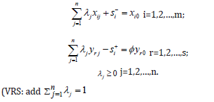
In the problem above, ϕ is a scalar that ranges between 1 and ∞. The inverse of ϕ ranges between 0 and 1 and is the technical efficiency score. If it is equal to 1, it implies that the DMU0 is efficient, if less than 1, the DMU0 is inefficient. Vector λ is a (n×1) vector of constants that measures the weights used to compute the location of an inefficient DMU if it were to become efficient. The model specification under the hypothesis of variable return to scale implies the condition of convexity of the frontier. This presumes that the restriction N1λ≤1 is introduced in the model, with N1 being an n dimensional vector of ones. The absence of this restriction would imply that returns to scale were constant. The DEA model is relatively simple to estimate but is deterministic and does not account for measurement error. The bootstrap approach must generally be combined with DEA to obtain statistical properties of the efficiency scores. The bootstrap is a computer intensive technique based on the idea of mimicking the unknown distribution of interest through the concept of resampling from the original sample. For more technical details on the DEA bootstrap method, see Simar and Wilson 2007.

Tobit regression model and multicollinearity tests

We use the Tobit regression technique to estimate the relationship between the efficiency variables according to the controlled models and the economic variables that predict efficiency. In this analysis, it is necessary to diagnose and control the multicollinearity tests using correlation coefficients, inflation variance factors and tolerance statistics. Tobit regression model, which was proposed by Tobin [48], describes the association between a non-negative dependent variable (latent variable) and independent variable(s) when the data is censored or truncated. The relative efficiency scores, which are obtained from the DEA models, range from 0.0 (left-censored) to 100.0 (right-censored). Hence, the Tobit model is an effective tool for the second stage of DEA analysis, because the data is censored from both the lower and upper bounds. The Tobit regression model can be formulated as

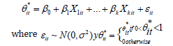
where β= (β₁,…,β_k ) is (k x 1), a vector of unknown coefficients which determines the relationship between what is a (1 x k) vector of independent variables (X₁,…,X_k)^tr and the latent (unobservable) variable θ*_it denotes the relative efficiency scores obtained from the DEA models, and ε_i t is a normally, identically and independently distributed error term. In this direction, DEA efficiency scores obtained in the first stage are used as a dependent variable in the second stage, one side censored Tobit model in order to allow for the restricted [0,100] range of efficiency values (Sufian & Noor, 2009). The simultaneous use of certain independent variables may lead to multicollinearity problems. We carry out two tests to check whether there is a potential multicollinearity problem in this study. First, we use variance inflation factors (VIFs) and tolerance statistic (TOL) to test for multicollinearity. As a rule of thumb, TOL should not be close to 0 and VIFs should not be greater than 10.

The dataset contains individual bank data sourced from statements of commercial banks operating in 21 EU member countries, as made available through the Bank Scope database of Bureau van Dijk. The period under study focuses on the aftermath of the 2007 crisis, 2011–2014, which involved a structural break for banks. Data have been scrutinized to avoid inconsistencies and to obtain a homogeneous dataset with 1588 observations García-Gil 2017. Data set of Economic Freedom is obtained from Heritage Foundation. The model proposed in this study follows the intermediation approach suggested by Berger [49]. Based on this, the outputs considered are earning assets (y1), investments in fixed and variable incomes in ownership of the entity, and loans (y2), the amount of customer loans (Casu [50]; Casu [51]; Chortareas et al. [15,16]). In addition, a third output takes into account several activities generating incomes from nontraditional banking sources. Barth et al. [52] consider this output not to penalize entities with a market share derived from non-traditional banking activities. Noninterest operating income (y3) constitutes an important fraction of the profit and loss statement of entities and has been included in recent studies (Moradi-Motlagh [53]; Moradi-Motlagh [54]). Other studies that agree on the selection of these three outputs are Ayadi [55]. As for inputs, the main model includes interest expense (x1), expenses derived from borrowed funds representing interest paid on any loans; and non-interest expense (x2), expenses assumed by an entity that do not form part of the financial expenses such as taxes, provisions, etc. (Sturm & Williams, 2004; Moradi-Motlagh [54]; Moradi-Motlagh [53]). includes customer deposits (x3), which represents the loanable funds; while alternative model B adds staff costs (x4), including salaries, allowances, social benefits and contributions Table 1. These inputs (x3) customer deposits and (x4) staff costs are selected in several recent studies: Chortareas et al., [16]; Koutsomanoli-Filippaki [56] and Ayadi et al. [55].

Table 1:Descriptive statistics for inputs and outputs.

The input x1 has gradually decreased with an average reduction of the interest expense of 30.54% in the period. Moreover, noninterest expenses, x2, presents a constant trend around 967.16 million euros, its average level for the period. The positive evolution of x3 means an increase of 7.84% of the average customer deposits in the period, while in the case of x4 the evolution is negative and implies a decrease of 3.87% in staff costs. As for outputs, the development of y1 and y2 shows a level decrease of 10.91% and 6.75% until 2013, respectively. From this year, their levels increased again reaching averages of earning assets and loans of 63469.27 and 33032.42 million euros respectively in 2014. As regards y3, the highest revenues from non-interest operations are obtained in 2012 (mean of 592.45 million euros). Since then, the evolution is declining to an average of 568.93 in 2014, representing a decrease of 3.97%. The economic freedom index and all its components are used to measure the influence of these variables on the inefficiency of banking institutions. These variables take values from 0 to 100, with the highest values indicating that the economic environment and the policies adopted favor economic freedom. Property Rights (PR) The property rights component is an assessment of the ability of individuals to accumulate private property, guaranteed by clear laws that must be fully enforced by the state. It measures the degree to which a country’s laws protect private property rights and the degree to which its government enforces the laws. It also assesses the likelihood that private property will be expropriated and analyzes the independence of the judiciary, the existence of corruption within the judiciary, and the ability of individuals and firms to enforce contracts.

Government Integrity (GI)

The score for this component is derived from Transparency International’s 2011 Corruption Perceptions Index (CPI), which measures the level of corruption in 183 countries. The CPI is based on a 10-point scale, where 10 indicates very little corruption and 0 indicates a very corrupt government. This index converts the raw CPI data into a scale from 0 to 100.

Government Spending (GS)

This component considers the level of government spending as a percentage of GDP. Government spending, including consumption and transfers, includes the entire score.t

Business Freedom (BF)

This is a global indicator of the efficiency of government regulation of business. The quantitative score is derived from a series of measures of the difficulty of starting, operating, and closing a business. The business freedom score for each country is a number between 0 and 100, where 100 equals the freest business environment. The score is based on 10 factors, all weighted equally, using data from the World Bank’s Doing Business study.

Labor Freedom (LF)

The labor freedom component is a quantitative measure that takes into account various aspects of the legal and regulatory framework of a country’s labor market, including rules regarding minimum wages, laws inhibiting layoffs, severance requirements, and measurable regulatory restrictions on hiring and hours worked. (Range: 0 to 100).

Monetary Freedom (MF)

Combines a measure of price stability with an assessment of price controls. Both inflation and price controls distort market activity. Price stability without microeconomic intervention is the ideal state for the free market. The score for the monetary freedom component is based on two factors: the weighted average inflation rate for the most recent three years and price controls (Range: 0 to 100).

Trade Freedom (TF)

A composite measure of the absence of tariff and non-tariff barriers affecting imports and exports of goods and services. The freedom of trade score is based on two inputs: the trade-weighted average tariff rate and Non-Tariff Barriers (NTBs). (Range: 0 to 100).

Investment Freedom (IF)

The index assesses a variety of restrictions that are typically imposed on investment. It follows that the ideal score is 100 for each of the restrictions found in a country’s investment regime. (Range: 0 to 100).

Financial Freedom (FF)

Measures independence from government control and intervention in the financial sector. High scores indicate high levels of financial freedom (Range: 0 to 100).

Economic Freedom (EF)

Is the fundamental right of every human being to control his or her own labor and property. In an economically free society, people are free to work, produce, consume and invest in whatever they want. In economically free societies, governments allow labor, capital, and goods to move freely, and refrain from coercion or restriction of freedom beyond the extent necessary to protect and maintain freedom itself. It is based on 10 quantitative and qualitative factors, grouped into four broad categories, or pillars of economic freedom. Each of the ten economic freedoms within these categories are rated on a scale of 0 to 100. Table 2 shows the descriptive statistics for the EF.

Table 2:Descriptive statistics for economic freedom variables.

The PR variable shows an increase in its average value at the beginning of the period from 75.50 in 2011 to 76.10 in 2012. From this year onwards, it decreases by 0.22% and remains stable until the end of the period. The maximum value reached by this variable is 90.00 and the minimum 40.00. The GI variable shows small increases and decreases in its value over the years with a reduction of 1.32% in the period analyzed. Its maximum and minimum values are 94.00 and 34.00, respectively. The averages of the GS and BF variables show a reduction in their levels of 21.21% and 0.93%, respectively, throughout the period, while the LF variable begins to increase its value from 2012, showing a growth of 5.31% between 2011 and 2014. The MF variable presents a negative annual variation rate of 2.98% in the period. Its maximum and minimum values are 83.90 and 72.40, respectively. Similarly, the LCOM variable reduces its levels by 5.50% until 2013. From that moment on, there is a turning point and it increased by 1.16% in the last year. The maximum and minimum values are 87.60 and 81.80, respectively. The IF and FF variables show a progressive growth of 5.95% and 1.95%, respectively, their average values being 81.02 and 70.60 in the 2011-2014 period for each of them. Finally, the EF variable, which is an average of all the previous variables, presents a decrease at the beginning of the period of 1.89%, increasing again in 2012 and remaining practically constant until the last year. The average value in the period is 68.91, with maximum and minimum values of 78.70 and 55.41, respectively.

As can be seen, the values of the averages of these variables are quite similar over the years. Likewise, the standard deviation of all of them is lower than their mean, so that the coefficient of variation presents values between 0.04 and 0.46, reflecting a high representativeness in the mean value of these variables. Table 3 shows the descriptive statistics for CAMELS model. The C ratio presents a positive variation rate every year from a value of 25.22% in 2011 to 29.73% in 2014, increasing by 17.88%. The average of this solvency indicator during the period is 28.01%. The average of the A ratio in the period is 68.94% manifesting an increasing trend until 2013, which represents an increase of 2.82%. From this moment on, it tends to decrease presenting a reduction in its value of 0.40%. With respect to this asset quality indicator, it can be said that the entities present low dispersion (variation coefficient 0.29) throughout the period, with a maximum value of 141.40% and a minimum value of 0%. The variable M experiences a decrease in its values from 3.08% in 2011 to 2.55% in 2014. Its maximum value is 133.33% and its minimum value is 0%. The coefficient of variation in the period is 2.00, indicating that the average (2.86%) is not representative. With respect to variable E, its maximum value in the period analyzed is 21.91% and its minimum value is -34.03%. The average of this variable increases every year (except in 2012), increasing its value from -0.09% in 2011 to 0.20% in 2014. The maximum value of the L variable is 1889.36% and the minimum is 0%. The average value is 95.43% with a coefficient of variation of 1.02. Over the years, a reduction in its average values of 4.03% is observed until 2013, where there is a change in trend and its value increases again in the last year. The behavior of the S variable over the period is stable. Throughout the years, its averages do not vary and are always 0.25%. Its coefficient of variation is 3.32.

Table 3:Descriptive statistics for CAMELS variables.

This section presents and discusses the empirical results of the efficiency model. Table 4 shows descriptive statistics for banking efficiency scores. The behavior of the average annual inefficiency is slightly increasing the first two years, obtaining a minimum in 2011 with 0.46 and a maximum in 2012 with 0.502. In 2013 and 2014, stability is maintained. The effects of CAMELS and EF in the regression model (year 2014) are shown in Table 5. Note that the dependent variable represents inefficiency, so the signs shown by the variables must interpret in a contrary to the studies of literature that analyze banking efficiency. With respect to economic growth, the increase in GDP has a positive coefficient in most cases, although it is only statistically significant in model 1. The result of the sign of the economic growth coefficient is in line with the results of previous studies. Pasiouras et al. [57], in their study of 95 countries, they find evidence of a negative relationship between technical efficiency and GDP growth. Chortaeas et al. [16] argue that entities that act in expanding markets can be less efficient controlling their expenses. Recently, Birir et al. 2017 find a negative relationship between GDP growth and efficiency explaining that high GDP growth causes low efficiency. In addition, Yildirim and Philippatos 2007 in their study on 12 economies in transition from central and east Europe during the 1993-2000 period, conclude a positive relationship of GDP growth with cost efficiency but find a negative relationship with efficiency in benefits. In contrast, there are also a series of studies that have a positive relationship of GDP with bank efficiency such as Lozano-Vivas and Pasiouras 2010.

Table 4:Descriptive statistics for inefficiency scores.

Table 5:The effect of camels model and economic freedom variables 2014.

When the models of economic freedom are included in the models, it is observed that the coefficients, the signs and the evolution in the behavior of the CAMELS system variables are similar to those found when the good governance indicators are included. PR shows a negative and statistically significant coefficient at 5%. This could indicate that the higher the protection of the country’s private property, lower, minors are the levels of inefficiency of its entities. In the banking sector of the European Union, inefficiency has been affected by the country’s property rights in the 2011- 2014 period. Similar results are found in recent studies such as Chortaeas et al. [16], which find a high positive relationship at the level of 1%, between this indicator and efficiency. Chortaeas et al. [16] argue that the entities present in countries with higher property rights have high levels of efficiency. On the other hand, Pasiouras et al. [57] find a positive relationship of the Government Property and Intervention Rights indices in economic activity with cost efficiency but find a negative relationship with benefit efficiency. The GI variable maintains a negative relationship with inefficiency, which could suggest that the higher the perception of freedom of corruption, minors will be the levels of inefficiency of the entities. This result is consistent with the achievement by inclusion of the good governance indicator in the previous models. Gaganis et al. [58] find a high positive coefficient at the level of 1% significance on efficiency, supporting the results found in this study. With respect to the GS variable, there is an absence of statistical significance throughout the period, although in most of the years it shows a coefficient with a negative sign, which could be interpreted as that entities that operate in countries with a higher expenditure index of the government, they have a lower inefficiency. The BF variable does not show influence on the inefficiency in any of the years analyzed although its coefficient presents a negative sign for most of them, which could suggest that the greater the business freedom of a country, the lower the level of inefficiency of the entities. Gaganis et al. [58] in their research obtain a positive and statistically significant relationship at the level of 1% between freedom of business and the efficiency of the entities. LF presents a positive and statistically significant relationship during all years with inefficiency, suggesting that the higher the level of labor freedom in the country, the lower the levels of inefficiency of the entities. The MF variable influences negatively (1%) in inefficiency in 2013, suggesting that higher levels of monetary freedom imply lower inefficiency. Likewise, the TF variable shows a negative and significant relationship with inefficiency in 2014, which could indicate that a greater absence of barriers to the country’s trade may allow entities to obtain minor inefficiency rates. IF also presents a negative and significant coefficient in the last two years, which could suggest that the higher the freedom of investment, the lower the level of inefficiency of the entities.

The FF variable is no significant relationship with inefficiency during the analyzed period, although over the years it shows a coefficient with a negative sign. This relationship could be interpreted as that entities present in countries with greater financial freedom tend to have minor inefficiency rates. Chortaeas et al. [16] suggest that the higher the country’s financial opening level, the higher the efficiency. In addition, Lin et al. [32] find that the foreign presence improves the efficiency levels of entities, especially in the case of countries where there is high financial freedom. Finally, the EF variable shows a negative relationship to the level of significance of 5% with the inefficiency in 2014, suggesting that the higher the level of economic freedom in the country, the lower the levels of inefficiency of the entities. C, measured by the level of institutions’ own resources among net loans, shows a decrease in its high significance (1%) on inefficiency during the second half of the period studied, reducing it to 10% in 2013 to recover partially again in the last year (5%). During the whole period, the ratio of C to bank inefficiency has ratios close to 0 and negative, suggesting that the higher the level of capitalization of the institutions to be able to cope with the provision of reserves and possible risk transactions carried out, the lower the levels of inefficiency. In addition, the higher this ratio, the more prepared the entities will be to be able to withstand potential financial crises and offer their customers greater security against adverse situations.

These results are similar to previous studies that determine the relationship between capital ratio and bank efficiency. Most of them measure capitalization as the level of own resources over the total asset, however, the following authors come to the same conclusions. Casu et al. [51] argue in their study on Italian financial conglomerates that the higher their capital ratio, the more efficient the entities will be. Chortareas et al. [15], on a sample of European Union commercial banks, reflect a negative sign of the ratio of the capital variable in the regression on banking inefficiency, suggesting that higher levels of capital are associated with greater efficiency. Chortareas et al. [16], in the second stage of the analysis of a sample of commercial banks from 27 Member States of the European Union, discover a positive relationship between capitalization and efficiency. Similarly, Sufian et al. 2016 find a positive relationship between this variable and efficiency in the Malaysian banking sector supporting the argument that well-capitalized institutions have a lower risk of bankruptcy. However, there are also studies that discover a negative and statistically significant relationship between capitalization and efficiency. This is the case of Batir et al. [59] which, on a sample of Turkish commercial banks, find a negative relation of this ratio with technical efficiency. The A ratio, calculated as the deposits among the total asset, has a high positive coefficient that reveals a significance of 1% during the whole period. This may indicate that the higher this ratio, which measures the quality of bank assets, the higher the levels of inefficiency because institutions have a greater share of their assets (including loans at risk of default) financed by customer deposits.

Similarly, variable M, which represents the quality of the management of institutions through interest expenditure among total deposits, shows a positive and significant sign over the years. For its interpretation it could be said that the higher the ratio, the higher the levels of inefficiency of the institutions since this would imply higher costs in terms of interest on the deposits with which they are financed. These results are in line with Batir et al. [59] that use this ratio and find a negative relationship with efficiency explaining that, entities that have high expenses may be using the inputs in excess and be less efficient. On the contrary, E, which measures the profitability of institutions over the average of the assets, has a negative and significant ratio at the level of 1% during the whole period, although in 2013 it reduced its significance to 10%. The fact that the relationship between the two variables is negative can be interpreted as that the institutions that present higher values for this ratio, are more profitable and benefit more in the levels of bank efficiency. These results are in line with Ariff [60], which find a positive but not significant ROA coefficient with efficiency, suggesting that higher profitability tends to be more efficient. Košak et al. [61] discover a negative relationship of ROAA with cost inefficiency. Sufian et al. 2009 shows a positive relationship between the ROA coefficient and the efficiency of the Islamic banking sector, indicating that the most efficient banks tend to be more profitable. In addition, studies analyzing another measure of profitability such as Chortareas et al. [16], obtain a positive and statistically significant sign of ROAE on the efficiency of entities from 27 Member States of the European Union. Similarly, Vu and Nahm 2013 find a positive effect of ROE on the profit efficiency of Vietnam’s banks during 2000-2006.

With respect to L, which measures liquidity risk through the relationship between total claims on deposits, it presents a negative ratio very close to 0 and statistically significant (1%) overall years. This implies that entities with high values of this ratio tend to have lower inefficiency rates. These results suggest that institutions can try to make the most of the funds obtained in order to present a lower inefficiency. Coinciding with these findings, Ariff [60] and Chortareas et al. [15]. Similarly, Řepková [62], in its study on the banking sector of the Czech Republic between 2001 and 2012, finds a positive and statistically significant ratio of loans between deposits with efficiency. Besides, Košak et al. [61], although they do not demonstrate a significant relationship between cost inefficiency and liquidity, they get the expected negative sign. Finally, the variable S, calculated as the bank assets of an institution among the total assets of the institutions of the banking system, also reveals a highly significant negative relationship (1%) with inefficiency over the period. This could indicate that, the higher the risk sensitivity ratio, the lower the inefficiency levels of entities. These results coincide with those of Košak et al. [61], those with a high significant and negative market share-to-cost inefficiency ratio of entities in five new Central and Eastern European Member States and the three Baltic States during the period 1996-2006. Grigorian [63], in their 1990 study on the banking sector of economies in transition, derive a positive relationship from this indicator with bank efficiency Figure 1.

Figure 1:Distribution by quartiles of economic freedom.

After carrying out this analysis by country, if one deepens the relationship of EF with inefficiency it is found that countries are in the highest quartiles of economic freedom (Ireland, 76.77; United Kingdom, 74.54; Finland, 73.57 and Sweden, 72.36), are present in the first quartile of inefficiency (0.44; 0,50; 0.38 and 0.48). In contrast, most countries in the first quarter of economic freedom (Greece, 56.64; Slovenia, 62.68; Poland, 65.09 and Portugal, 63.29), are framed in the highest quartiles of inefficiency which shows an influence of economic freedom on it [64]. This result coincides with the negative relationship explained in the inefficiency models previously estimated. As an exception we can find on the one hand Denmark, which reaches high values of this variable and inefficiency (76.76) and on the other, France and Italy with low averages for economic freedom and inefficiency (64.00 and 60.07, respectively). Finally, the Nordic countries Finland and Sweden are identified as the countries with the greatest economic freedom (Q4 in GI, BF, EF). In addition, Sweden excels in quartile 4 of MF and IF, while Finland excels in quartile 1 of LF. Other countries to be highlighted are the United Kingdom in the fourth quarters of BF, IF and EF and Ireland in the last two. Likewise, the average inefficiency levels of its banks are in the first quartile. On the other hand, the economies in transition together with Greece are in the first quartiles of the variables of economic freedom, presenting in turn high levels of inefficiency. Specifically, Slovenia and Greece in the first quartile of PR, IF and EF, highlighting the latter also in BF and MF. Slovakia and Poland have low BF and high LF values, and Poland stands out in the last quartiles of MF, IF and EF.

In an arduous economic environment, preceded by the financial crisis of 2008 and the subsequent Great Recession, the study on the ability of bank managers to cope with the aftermath of the crisis and the analysis of the influence that the country’s political framework has on banking behavior, are issues of permanent interest. Although not unanimous, most studies report that banks belonging to countries with quality governments and competitive institutions manage their resources with higher levels of efficiency. This research contributes to the debate that compares the efficiency of European banks during a period of political upheaval, from 2011 to 2014, when the aftermath of the Great Recession occurred. There is a long succession of studies analyzing European banking efficiency and the macroeconomic, institutional, financial and bank-specific determinants. However, the evidence contained in this article demonstrates the significant influence of economic freedom and its dimensions, in addition to CAMELS variables, on bank efficiency.

In this sense, this research reports that increases in capital requirements and a greater ability to generate profits favors bank efficiency. However, there is no consensus on the effect of the liquidity ratio. In particular, it is concluded that banks are trying to achieve the highest return on available funds to increase efficiency. In terms of asset quality, the improvement of deposits in total assets has a positive effect on efficiency and the results on expenditure show that institutions with high interest charges in respect of deposits are less efficient. Close to market risk sensitivity, this work confirms the association of a higher commission on assets with a lower inefficiency of banks. The study of bank efficiency reveals significant differences by country in the sample analyzed. Among the least efficient institutions are banks located in economies in transition such as Hungary, Denmark, Slovakia, Slovenia and Poland. On the contrary, among the most efficient are banking systems in Finland, Ireland, France, Spain, Sweden and the United Kingdom. In addition, there is an association between the distribution of the efficiency of banking systems and the ranking according to the economic freedom of the country where they are located. In line with the results, the politicians of the economies in transition should make an effort to increase the levels in the dimensions that define economic freedom and thus, by removing institutional restrictions, facilitate the possibility of a more efficient banking management.

1. Barth J, Caprio G, Levine R (2013) Bank regulation and supervision in 180 Countries from 1999 to 2011. Journal of Financial Economic Policy 5(2).
2. Taboada AG (2011) The impact of changes in bank ownership structure on the allocation of capital: International evidence. Journal of Banking & Finance 35(10): 2528-2543.
3. Michalak CT, Uhde A (2012) Credit risk securitization and bank soundness in Europe. The Quarterly Review of Economics and Finance, Elsevier 52(3): 272-285.
4. Elliott JD, Greg F, Andreas L (2013) The history of cyclical macroprudential policy in the United States of financial research Working Paper No. 8 (Washington: U.S. Department of the Treasury).
5. Slimane FB, Mehanaoui M, Kazi IA (2013) How does the financial crisis affect volatility behavior and transmission among European stock markets? Int J Financ Stud 1(3): 1-21.
6. Barucci E, Baviera R, Milani C (2014) Is the comprehensive assessment really comprehensive? SSRN Electronic Journal.
7. Bokpin GA (2013) Ownership structure, corporate governance and bank efficiency: An empirical analysis of panel data from the banking industry in Ghana. Corporate Governance 13(3): 274-278.
8. Alhassan AL (2015) Income diversification and bank efficiency in an emerging market. Managerial Finance 41: 1318-1335.
9. Fujji H, Matousek R, Rughoo A (2017) Bank efficiency, productivity, and convergence in EU countries: A weighted Russell directional distance model. The European Journal of Finance 24(2): 1-25.
10. Arun T, Turner J (2004) Corporate governance of banks in developing economies: Concepts and issues. Corporate governance: An International Review 12(3): 371-377.
11. Kablan S (2017) Banking efficiency and financial development in sub-Saharan Africa.
12. Fries S, Taci A (2005) Cost efficiency of banks in transition: Evidence from 289 banks in 15 post-communist countries. Journal of Banking & Finance 29(1): 55-81.
13. Kasman A, Yildirim C (2006) Cost and profit efficiencies in transition banking: the case of new EU members. Applied Economics 38(9): 1079-1090.
14. Andries AM (2011) The determinants of bank efficiency and productivity growth in the central and eastern European banking systems. Eastern European Economics 49(6): 38-59.
15. Chortareas G, Girardone C, Ventouri A (2012) Bank supervision, regulation, and efficiency: Evidence from the European union. Journal of Financial Stability, Elsevier 8(4): 292-302.
16. Chortareas G, Girardone C, Ventouri A (2013) Financial freedom and bank efficiency: Evidence from the European union. Journal of Banking & Finance 37(4): 1223-1231
17. Tsionas EG, Assaf AG, Matousek R (2015) Dynamic technical and allocative efficiencies in European banking. Journal of Banking & Finance, Elsevier 52(C): 130-139.
18. Chen, Hsuan-Chi C, Chia-Wei Y (2021) Global financial crisis and COVID-19: Industrial reactions. Finance Research Letters 42: 101940.
19. Abreu A (2021) Innovation ecosystems: A sustainability perspective. Sustainability 13(4): 1-3.
20. Aliyu A, Modu B, Tan C (2017) A review of renewable energy development in Africa: A focus in South Africa, Egypt and Nigeria. Renewable and Sustainable Energy Reviews 81(2): 2502-2518.
21. Bhatia A, Siya T (2018) Sustainability reporting: An empirical evaluation of emerging and developed economies. Journal of Global Responsibility 9(2).
22. Lopes JM, Gomes S, Oliveira J, Oliveira M (2021) The role of open innovation, and the performance of European union regions. J Open Innov Technol Mark Complex 7(2): 120
23. Adkins L, Moomaw R, Savvides A (2002) Institutions, freedom and technical efficiency. South Econ J 69(1): 92-108.
24. Bergh A, Karlsson M (2010) Government size and growth: Accounting for economic freedom and globalization. Public Choice 142(1): 195-213.
25. Heckelman JC, Knack S (2009) Aid, economic freedom and growth. Contemp Econ Policy 27(1): 46-53.
26. Claessens S, Laeven L (2004) What drives bank competition? Some international evidence. J Money Credit Bank 36(3): 563-583.
27. Sufian F, Habibullah MS (2012) Globalization and bank performance in China. Res Int Bus Financ 26(2): 221-239.
28. Bjornskov C (2016) Economic freedom and economic crises. Eur J Polit Econ 45: 11-23.
29. Asteriou D, Pilbeam K, Pratiwi CE (2021) Public debt and economic growth: Panel data evidence for Asian countries. Journal of Economics and Finance, Springer; Academy of Economics and Finance 45(2): 270-287.
30. Holmes KR, Feulner EJ, O Grady MA (2008) Index of economic freedom. Heritage Foundation.
31. Blau B (2017) Economic freedom and crashes in financial markets. Journal of J Int Markets Inst Money 47: 33-46.
32. Lin KL, Doan AT, Doong SC (2016) Changes in ownership structure and bank efficiency in Asian developing countries: The role of financial freedom. Int Rev Econ Financ 43: 19-34.
33. Betz F, Oprica S, Peltonen TA, Sarlin P (2014) Predicting distress in European banks. Journal of Banking and Finance 45: 225-241.
34. Mayes D, Stremmel H (2012) The effectiveness of capital adequacy measures in predicting bank distress. Financial Markets & Corporate Governance Conference, p. 46.
35. Rebel AC, White L (2012) Déjà vu all over again: The causes of US commercial bank failures this time around. Journal of Financial Services Research 42(1-2): 5-29.
36. Berger A, Bouwman H (2013) How does capital affect bank performance during financial crises? Journal of Financial Economic 109(1): 146-176.
37. Vazquez F, Pablo F (2015) Bank funding structures and risk: Evidence from the global financial crisis. Journal of Banking & Finance 61: 1-14.
38. Cole RA, White LJ (2011) Déjà vu all over again: The causes of US commercial bank failures this time around. Journal of Financial Services Research 42: 5-29.
39. Chiaramonte L, Croci E, Poli F (2015) Should we trust the z- score? Evidence from the European banking industry. Global Finance Journal 28: 111-131.
40. Poghosyan T, Čihák M (2009) Distress in European banks: An analysis based on a new dataset. IMF working papers, pp. 1-37.
41. Mayes D, Stremmel H (2012) The effectiveness of capital adequacy measures in predicting bank distress. Financial Markets & Corporate Governance Conference, p. 46.
42. Messai AS, Gallali MI (2015) Financial leading indicators of banking distress: A micro prudential Approach- Evidence from Europe 11(21).
43. Cole RA, Wu Q (2017) Hazard versus Probit in predicting U.S. Bank Failures: A Regulatory Perspective over Two Crises.
44. Wanke P, Azad AK, Barros CP, Hadi-Vencheh A (2015) A predicting performance in ASEAN banks: An integrated fuzzy MCDM-neural network approach. Expert Systems 33(3): 213-229.
45. Roman A, Sargu AC (2013) Analyzing the financial soundness of the commercial banks in Romania: An approach based on the Camels framework. Procedia Economics and Finance 6: 703-712.
46. Wanke P, Azad MAK, Barros CP (2016) Financial distress and the Malaysian dual baking system: A dynamic slacks approach. J Bank Finance 66: 1-18.
47. Rozzani N, Rashidah R (2013) Camels and performance evaluation of banks in Malaysia: Conventional versus Islamic. Journal of Islamic Finance and Business Research 2: 36-45.
48. Tobin J (1958) Liquidity preference as behavior towards risk. The Review of Economic Studies 25(2): 65-86.
49. Berger AN, Humphrey DB (1997) Efficiency of financial institutions: International survey and directions for future research. European Journal of Operational Research 98(2): 175-212.
50. Casu B, Molineux P (2003) A comparative study of efficiency in European banking. Appl Econ 35(17): 1865-1876.
51. Casu B, Girardone C (2004) Financial conglomeration: Efficiency, productivity and strategic drive. Appl Fin Econ 14(10): 687-696.
52. Barth JR, Lin C, Ma Y, Seade J, Song FM (2013) Do bank regulation, supervision and monitoring enhance or impede bank efficiency? Journal of Banking & Finance 37(8): 2879-2892.
53. Moradi-motlagh A, Babacan A (2015) The impact of the global financial crisis on the efficiency of Australian banks. Econ Model 46: 397-406.
54. Moradi-Motlagh A, Saleh AS (2014) Re-examining the technical efficiency of Australian banks: A bootstrap DEA approach. Austral Econ Papers 53(1-2): 112-128.
55. Ayadi R, Naceur SB, Casu B, Quinn B (2016) Does Basel compliance matter for bank performance? J Financ Stability 23: 15-32.
56. Koutsomanoli-Filippaki A, Mamatzakis E, Pasiouras F (2013) A quantile regression approach to bank efficiency measurement. Efficiency and productivity growth: Modelling in the financial services industry.
57. Pasiouras F (2008) Estimating the technical and scale efficiency of Greek commercial banks: The impact of credit risk, off-balance sheet activities, and international operations. Research in International Business and Finance 22(3): 301-318.
58. Gaganis C, Pasiouras F (2013) Financial supervision regimes and bank efficiency: International evidence. Journal of Banking & Finance 37(12): 5463-5475.
59. Batir ET, Volkman DA, Gungor B (2017) Determinants of bank efficiency in Turkey: Participation banks versus conventional banks. Borsa Istanbul Review 17(2): 86-96.
60. Ariff M, Can L (2008) Cost and profit efficiency of Chinese banks: A non-parametric analysis. China Economic Review 19(2): 260-273.
61. Kosak M, Zajc P, Zoric J (2009) Bank efficiency differences in the new EU member states. Balt J Econ 9(2): 67-89.
62. Řepkova I (2015) Banking efficiency determinants in the Czech banking sector. Procedia Econ Finance 23: 191-196.
63. Grigorian DA, Manole V (2002) Determinants of commercial bank performance in transition-an application of data envelopment analysis. Comp Econ Stud 48(3): 497-522.
64. Ayadi R, Ben NS, Casu B, Quinn B (2015) Does Basel compliance matter for bank performance?