Stochastic Distribution Control Theory-Its Potential Application in Risk Management in Financial Systems

In finance and accounting systems, evaluation of control of risk has always been a subject of study [2,3] with reference therein. Risk analysis and management require a good understanding of the quantitative relationships between the risk and the key factors that influence the concerned risk. It is a dynamic stochastic system where the inputs are the identified factors that affect the risk whilst the output is the risk represented as a random process. For example, value at risk (VaR) is a random process that can be used to predict the maximum possible losses over a specific time duration [2]. The factors that affect VaR are generally the period, confidence level and the size of possible losses which can be affected by random disturbances. Indeed, since these factors can be of random nature, the system dynamics shall be represented by stochastic differential equations such as Ito stochastic differential equations or time-series models in discretized-time domain format that are subjected to random disturbances. This means that the management (or the control) of the risk would require the following:
1) Development of risk propagation models that link the risk with the key inputs.
2) Optimize a subset of inputs in their capacity as decision or control variables so that the risk can be minimized in the concerns precision zone at high confidence level.

The first requires a good model to be developed and the second aspect is basically the objective of risk management or control. As discussed before, the risk models are either of the format as stochastic differential equations or the time series models subjected to random disturbances. These models reveal how the risk, as a random process calculated for example as VaR, is affected by various factors. However, these existing models are mostly assumed to be subjected to Gaussian inputs and they are limited when dealing with non-Gaussian cases widely seen in practice. In this review, we will discuss potential applications of stochastic distribution control theory to the risk analysis and management. For this purpose, in the next section we will brief introduce the concept of stochastic distribution control. In particular we will explore how such a theory can be applied to deal with non-Gaussian risk management systems in general.

Stochastic distribution control

Given a stochastic system, its model is defined as a set of mathematic equations that represent the relationship between the inputs and outputs. In risk management, the risk under consideration would be the output whilst the inputs are the factors that affect the estimation and management (and control) of the risk. In general risk is measured as an event probability as it is normally affected by some random disturbances and noises. Since the probability density function is a comprehensive measure of the characteristics of any random variable, the objective of stochastic distribution control is to find out a set of inputs so that the output probability density functions can be made to follow a targeted distribution shape. The theory of SDC was originated in 1996 by the author [1,4,5]. Since then, numerous modeling and control strategies have been developed and applied to many engineering systems. Indeed, it has been shown that the SDC theory can effectively deal with non- Gaussian systems and is therefore much generic than traditional stochastic system theory in which only mean and variance of the system output are controlled or managed. In terms of the modeling in SDC theory, a decoupled expression is often used based upon the universal approximation properties of neural networks such as B-splines neural networks [1], where the output PDF of the system is approximated and learned using a neural network and the system dynamics is represented as a set of dynamic equations (often differential equations) that links the inputs to the weights of the neural network that approximates the output PDF of the concerned system. When the output PDF cannot be measured, a generical input-output model is obtained first, and the relationship between the output PDF and the inputs is then formulated using the well-known chain formula in probability theory. Using such a set of PDF models one can design and manipulate inputs so that the output PDF can be controlled. In the next section, we will describe how risk management can be well handled by SDC theory as a potential direction of research in the future.

Risk management using SDC

Denote 𝑟(𝑘) as a value of risk at a sample-time instant 𝑘 and assume that it is affected by a set of factors denoted by 𝑢(𝑘) ∈ 𝑅𝑛 as an n-dimensional vector, then in general one can use the following model, that links the inputs to the output (i.e., VaR), to represent the system.

where 𝑓(… ) is a generic function that can be learned using historical data of the concerned system, 𝑚 is an integer that defines the dynamic order of the system, and 𝜔(𝑘) is a random disturbance process that makes the VaR a random process as well. With this model in mind, the risk analysis would mean to find out function 𝑓(…) and then use inputs with this function to calculate VaR for future discrete time instants say 𝑟(𝑘 + 1) when the current time instant is 𝑘. As it is the author’s believe that in general VaR is a random variable, one can denote the probability density function of the value at risk 𝑟(𝑘 + 1) as 𝛾(𝑥), with 𝑥 ∈ [0, +∞) as the index variable in the definition interval [0, +∞), then this PDF would be generally a conditional PDF with respect to the past observed VaRs and the relevant factors 𝑢(𝑘) at the current sample instant 𝑘. This means that the PDF of VAR at sample instant 𝑘 + 1 can be expressed as γ (x | r(k),..., r(k −m),u(k)) . This means that the probability of the value at risk larger than a given threshold 𝜋 > 0 at sample instant 𝑘 can be expressed as a conditional probability of the following form.

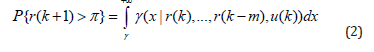
In this scenarios, it has been assumed that the past observed values at risk are available for the calculation and justification. As stated in section 1, the relationship between function (…) and PDF 𝛾(𝑥) can be obtained using the following well-known chain rule in the probability theory.

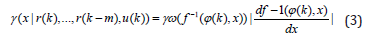
where it has been denoted that 𝜑(𝑘) = [𝑟(𝑘), …, 𝑟(𝑘 − 𝑚) 𝑢(𝑘)] 𝑇 and 𝛾𝜔(𝑥) is the probability density function of the random disturbance process 𝜔(𝑘). 𝑓-1(𝜑(𝑘), 𝑥) is an inverse map of 𝑓(𝜑(𝑘), 𝜔(𝑘)) with respect to the entry position of 𝜔(𝑘) under the assumption that 𝑓(𝜑(𝑘), 𝜔(𝑘)) is monotonic with respect to 𝜔(𝑘) [4]. It can be seen from equation (2) that the risk is measured as a probability of its value larger than a certain number or threshold. In this context, equations (1) and (2) present a generic description of risk analysis and management. Indeed, a good management of risk would be to have its VaR’s PDF as narrow and as left as possible in its PDF plot as shown in the following figure. In the above figure, the good PDF of VaR means that its mean value is small and its variance (entropy) is small - showing that the uncertainties embedded in calculating VaR is small. In an extreme case the PDF of a VaR is an impulse function centered at zero, then the risk is of course zero and the system concerned does not any risk in its operation. This observation says that in terms of risk management, a good management strategy is to control the shape of 𝛾(𝑥|𝜑(𝑘)) so that it approaches an impulse PDF centered at zero. This requires the solution of the following optimal risk management strategies.

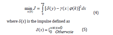
Equation (4) means that to achieve the lowest possible VaR at discrete sample instant 𝑘 + 1, we need to make sure that the PDF 𝛾(𝑥|𝜑(𝑘) is made as close as possible to a special PDF shape defined by the impulse function. Once the optimization problem in equation (4) is solved, a good PDF of VaR as shown in Figure 1 can be readily obtained – leading to an optimized risk management strategy with high confidence. Indeed, to focus on the high confidence effect, one can simply consider to minimize the entropy of VaR. This can be realized by solving the following optimization problem.

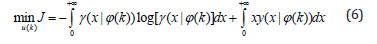
Figure 1:The PDF of VaR at sample instant 𝑘 + 1([4]).

where the first term in equation (6) is the entropy of VaR and the second term is its mean value. Since the entropy is a measure of randomness in VaR, its minimization would be to obtain the high confidence estimate of VaR, whilst the mean minimization indicates a low risk effect by using optimized decision inputs (factors).

In the author’s opinion, risk analysis and management are in line with the scope of stochastic distribution control theory, where the modeling of VaR in the structure of equation (1) needs to be performed first in order to reveal the quantitative relationship between VaR and the input factors. This is a modeling exercise where data driven modeling and neural network based approaches can be used. Once such a VaR model is obtained, the risk management would be to control the inputs so that the PDF of the VaR can be shaped to be as close as possible to an impulse PDF defined in equation (5). As such, the concerned risk can be minimized with high confidence. In conclusion, one can use the comprehensive tools developed in stochastic distribution control to perform effective risk analysis and management. These would lead to future directions of research in this area, and further studies on the enhancement of robustness of the risk modeling and management strategies will be expected.

1. Wang H (2000) Bounded dynamic stochastic distributions, modeling and control, Springer-Verlag, London, UK.
2. Filusch T (2021) Risk assessment for financial accounting: Modeling probability of default. Journal of Risk Finance 22(1): 1-15.
3. Bilir H (2016) Value at Risk (VaR) measurement on a diversified portfolio: Decomposition of idiosyncratic risk in a pharmaceutical industry. European Journal of Business and Management 8(6): 2016.
4. Guo L, Wang H (2010) Stochastic distribution control systems design: A convex optimization approach, Springer-Verlag, London, UK, p.191.
5. Wang A, Wang H (2021) Survey on stochastic distribution systems: A full probability density function control theory with potential applications. Optimal Control Applications and Methods 42(6): 1812-1839.