Advances in Modern Portfolio Theory

The portfolio theory started its formalization from the simple definition of mean asset returns and covariance matrix as risks of assets and their mutual influence between the asset returns. This formal background was named Mean-Variance (MV) theory and it is widely used for comparison reasons between different modification and complications of portfolio problems [1-5]. The main task of the portfolio management is the optimal resource allocation per different assets in the portfolio. Thus, the goal of this portfolio management is to obtain maximal portfolio return, keeping minimization of the portfolio risk for the end of an investment period. The formal presentation of the portfolio management concerns definition solution of appropriate portfolio optimization problems [6-8]. The formal complications of the portfolio theory concern additional inclusions of different parameters and relations, which are added to the portfolio problems. The MV model of the portfolio theory applies quantification of the asset’s characteristics: mean asset returns, evaluation of the covariance matrix of the asset returns. This formal portfolio problem sequentially is complicated by different types of definition of assets returns and assets risks. The portfolio theory complicated the content of the asset returns by different categories of returns as “current return values” [9,10], “mean values” [6], “implied values” [11,12]. The formal definitions of the risk applied are used under deterministic and probabilistic definitions as ‘’variance/covariance” between the assets returns [9] and “Value at Risk” (VaR) and its derivatives as “Conditional VaR” [13,14]. The complications of the portfolio theory address not only portfolio parameters, but introduce additional formal relations, derived from the investment process. Except the classical analytical relations of the MV model [9], additional relations are derived by the Capital Asset Pricing Model (CAPM) [15]; the Black-Litermman (BL) model includes additional relations, which formalize the inclusion of subjective assessments about the assets parameters [16-19]. The portfolio problem can be defined formally with different mathematical structure and containing different set of constraints: portfolio problem for one period of investment; multiperiod portfolio optimization; constraints with linear, nonlinear and/or integer relations. The majority of the portfolio problems apply only one goal function for the optimization of the resource allocation. A new complicated form of optimization currently is under experimentation which applies hierarchical, multilevel, particularly bi-level optimization. It allows the portfolio problem to be defined with more than one goal function and the assets allocation will satisfy additional requirements except for risk and return [3].

Advances in portfolio definition

The modern portfolio theory starts with quantitative assessment of the asset characteristics. The common parameters, evaluated as asset characteristics are the mean asset returns, the risk of each asset and the relations between the asset returns. The last two sets of asset characteristics quantitatively are given with the covariance matrix between the asset returns [4,20]. These quantitative portfolio characteristics are used for the definition of the classical portfolio problems [6].

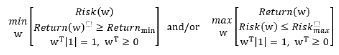(1)

where

w = (w₁,…,w_N)^T is the vector of weights, giving the relative value of the investment, allocated to asset i, i=1,N- number of assets in the portfolio;

Relation requires the investment amount to be totally allocated to the portfolio.

w≥0 means that the assets are bought for the portfolio.

Risk (w) and Return (w) are analytical functions with the portfolio solutions w.

(Return)_min And (Risk)_max are predefined values, required for the portfolio problem.

 The function Return ( ) analytically is defined as weighted sum of the asset returns

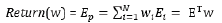(2)

where E_i is the mean asset return for a period t∈ [0, T], evaluated from the historical data of the real assets returns   Rⁱ_t, i = 1, N, t=[0,T]. The analytical relation between E_i and Rⁱ_t is 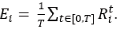  The portfolio risk σ_p is given by the standard deviation of the portfolio return E_p. The analytical definition between the asset risks s_i and the covariance coefficients σ_ij, i, j=1, N is

where (3)

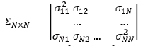is a symmetric matrix and its main diagonal contains the values of the assets risk σ_ii². The components of Σσ_ii² are evaluated as

(4)

The portfolio problem can be modified by definition of the portfolio goal function for simultaneously maximization of the portfolio return and minimization of the portfolio risk

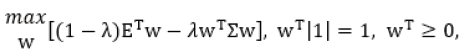(5)

where the coefficient λ∈ [0,1] defines the relative ability of the investor to undertake risk. For the case λ=0 the investor targets maximization of return without considering the portfolio risk. On the other boundary λ=1 the portfolio gives only minimization of risk. If (5) is solved with different values of λ, the solution w(λ) defines different values of the portfolio return E^Tw(λ) and risk w^TEw(λ). These values give a set of points in the space Return (Risk). Graphically, in this space a convex curve is presented, which is titled “efficient frontier”. The investor is recommended to choose one point from the “efficient frontier”, which will give the solution of his portfolio problem: w, Risk(w), Return(w). It is obvious, that the solutions of (5) strongly depend on the assets parameters E and Σ. The correct definition of them is a prerequisite for useful evaluated solutions w. Because the investment process can use only currently and historical data about the assets, and the portfolio results depend on the future levels of the portfolio assets, this methodological complication of the investment process insists forecasting of the future asset characteristics for the end of the investment horizon [10,20]. The portfolio theory pays special attention for the correct estimation and forecasting of the portfolio parameters: mean asset returns and covariance [10,21]. The accuracy of this estimation is a prerequisite for beneficial and successful application of the portfolio decisions [3]. The main assumption in the portfolio theory is that the asset characteristics will preserve its values till the end of the investment horizon [22]. That is why the correct forecast and identification is under the scope of several identification procedures [21]. The approaches ARMA and GARCH give formal background for the estimation of the future levels of asset returns. The ARMA relations contain two components: Auto Regressive (AR) and Moving Average (MA). The AR component evaluates the current asset return considering the values of its past levels

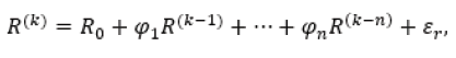
where Ro is the basic level of return and R^(k−n) are its past values, n is the length of the historical period, k is the current discrete time, ϕ_n are weighted coefficients for inclusion the past values, ε_n is the market noise. Such formal relation is appllied to estimate a future asset return considering the current trend in history period for its behavior. A peculiiarity of the AR modeling requires a big set of data about the historical behavior of the asset return. An additional complication for this model is the necessity of definition of the weighted coefficients ϕ_n. For the MA modeling, the idea is to assess the errors ε between the real historical data and the provided forecasts

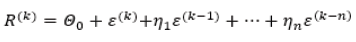
This modeling also suffer from the needs to keep long set of historical data and estimations as realistic motivation for the choice of the weighted coefficient η_n. Currently, the most used formal relations of ARMA are in the form ARMA (1,1), which means the usage only the current and previous value of the asset return and/or estimation errors. Another methodology for forecasting is GARCH, applied for evaluation of asset risk σi and covariances σ_i,j. GARCH abbreviation means General Auto Regressive Conditional Heteroscedasticity process [23]. The formal relation of GARCH is given as

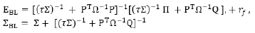
where σ concerns both asset risk σi and covariance components σ_i,j. The basic value σ_o and the weighted coefficient α_p, β_q must be additionally defined, which complicates the usage of GARCH. The methodology of GARCH in practical applications is also used for short historical period, p=q=1, GARCH (1,1) [24]. A next theoretical achievement of the modern portfolio theory is the development of Capital Asset Pricing Model (CAPM) [25]. This model introduces new portfolio parameters: the existence of market portfolio and its portfolio parameters as market return E_M and market risk σ_M. These market parameters have been formally related to the portfolio characteristics and new relations have been derived as:

1.The “Capital Market Line” (CML) which gives analytical description between the portfolio mean return E_p, portfolio risk s_p, the market parameters E_M, s_M and the risk free return r_f, . This line gives values about the possible portfolio returns and risks on the particular market (E_M, s_M) and risk free level r_f.

2.The “Characteristic line” (HL), which gives analytical relation between the current values of the market return R_M and the current asset return . This relation can be used to forecast the asset returns, according to the current level of the market return R_M.

3.The “Security Market Line” (SML) gives relation between the mean asset return E_i and the market characteristics E_M, s_M, r_f.

All these formal relations can be applied for the assessing an arbitrary portfolio return and risk for particular market (CML); to estimate future level of asset mean return for the particular market (SML); to relate the current value of asset return according to the market one. Because in practice the market parameters are defined by the market indices, the CAPM allows to be evaluated the parameters of the portfolio optimization problem. A complication for the definition of the portfolio risk is made by introducing its probability definition. The new risk parameter is named Value at Risk (VaR) and it its development is described in [9,26]. The VaR parameter quantifies the maximum like loss for the next trading day. It is evaluated using the deviations and correlations between the asset returns [4,14]. The VaR evaluation now is widely applied for risk management, which gives major positive effect [13]. VaR is developed and regarded as a component of the Portfolio theory.

Both the classical portfolio problem and the CAPM use historical values of the asset returns to evaluate the portfolio parameters. A new model, derived by Black-Litterman (BL), introduces a new set if initial data for the estimation and forecasting the asset parameters [16,17,27,28]. The new source of data comes for subjective expert views, which can set directly new values of the asset returns or to define relative assessment about them. The relative assessment gives data in percentage about the increase or decrease of the return of asset i towards asset j. The BL model allows to be integrated the historical data of asset returns and the subjective expert forecasts for evaluation of the asset return and risk characteristics [12,18, 29,30]. The BL model introduces new formal relations to incorporate the subjective views to the assets characteristics. An important component of the BL model is the introduction of new types of returns, named “implied returns”, П_i, i=1, N. These returns p_i are evaluated according to the market characteristics E_M,s_M. These new “implied returns” with the formal definition of expert views, matrices P, Q modify the mean asset returns  and the covariance matrix 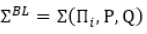. The BL model makes modification of the parameters of the portfolio problem and its solution differ from the solution of the classical portfolio problem, according to the inclusion of expert views for the future asset returns.

Description of peculiarities of black-litterman model

The BL model integrates historical data of asset returns with forecast of expert views [11,16,31,32]. The formal evaluations of the asset characteristics are presented graphically in Figure 1. The views are formalized with numerical new matrices П,P, Q, Ω and a coefficient τ . One can find estensive explanations of the BL model in [29,31]. The evaluation of the asset returns gives new matrices E_BL, S_BL which are used in the portfolio problem (5). The solution of (5) gives new weights W_BL in comparison with the initial case with w for the asset weights. The relations, which modify the parameters E_BL, S_BL in the BL model are:

Figure 1:Graphical interpretation of sequence of evaluations for BL model.

(6)

γ_f is the return of risk free asset, E, Σ are evaluated only from historical source of information for the evaluation of the asset characteristics, according to (2-4). The vector П contains the new set of “implied returns”. Relations (6) has also the set of new parameters, for the expert views P, Q, Ω, τ. The sequences for evaluation of these new parameters are the followingg: The “implied returns”are evaluated from the relation

(7)

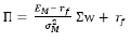
where the market parameters of the “market portfolio” are used, defined by the CAPM [24]. The matrices P,Q formalize quantitatively the values of the expert views. The example below says

that the first row of P gives forecast that the second asset will have Q(1)= 3% return. The second row of P gives forecast that the fourth asset return P(2,4)=1 will outperform the first one P(2,1)= -1 with Q(2)= 4%. The matrix Ω quantifies and in common is evaluated as diagonal matrix Ω = τ diag (PΣ P^{T>). The coefficient τ<1 is kept small and can have values, related to the duration n of the historical period, τ = 1/n [11]. The coefficient must decrease the value of the evaluated covariance matrix Σ with historical data of the asset returns. This research illustrates the usage of the classical portfolio theory, here defined by problem (6) and the modifications, applied by the BL model. The addded value of this research is the implementation of sliding procedure for definition and solution of portfolio problems. This procedure allows dynamically to manage the investments in time. The second peculiarity of this paper is the untroduction a special formalization of the matrix P of the expert views in BL model. This formalization allows to be used the historical data about the asset returns and to estimate additional information for the definition of P. Such formalization allows to be compared the solutions of the portfolio problems, solved with historical and BL data, because both problems are defined with common set of innitial data. The benefit of the portfolio solutions are assessed according to the content of the portfolio solutions w of the classical portfolio model and the solutions w_BL of BL model.}

Sliding procedure for active portfolio management

The paper illustrates application of active portfolio management. The content of this management concerns application of sliding procedure for definition and solution of appropriate portfolio problems. Each problem is defined with historical data of fixed previous period. Its solution is compared with the real results for the next time period. Then, a sliding move with the historical data is performed by dropping the last data and including new ones from the next period. This active management is implemented with two portfolio models: classical one, using only historical data and BL one, where additional corrections for the portfolio parameters are done. The active management is illustrated with data of the real estate market in Bulgaria. The National Statistical Institute of Bulgaria currently follows the prices of real estates on National level and evaluates indices named House Price Indices (HPI) [33]. The HPI indices contain data about new dwellings, mainly apartments (“New”) and currently trading estates (“Old”). The HPI indices are given also in the relative form about the change of the current HPI value in comparison with its previous one. Thus, HPI index gives the return of the estates, compared with the previous index evaluation. Each value of the HPI is calculated for a three month period, which gives four points per year. On Figure 2 is illustrated example of the HPI data. The graphical interpretation of these data is given in Figure 3 for illustration because it is not evident which asset “New” or “Old” is preferable for investment. This recommendation will be evaluated with the portfolio theory. The sliding mode of active management is defined according to three months historical data. Using these historical data the asset parameters E= (E_i, i=1,2) and covariance matrix Σ are calculated. The defined portfolio problem (6) is solved multiple time with different values of λ∈ [0,1], which gives numerical points of the “efficient frontier”. The portfolio, which is recommended for investment is chosen according to the maximal value of the Excess Sharpe ratio

Figure 2: Example of the HPI data.

Figure 3:The historical behavior of the HPI returns for “New” and “Old” estates.

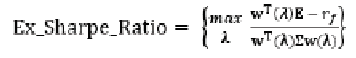(8)

The corresponding weights W^opt= [W^opt_New, W^opt_old]^T are also found. The comparison between the components and determines the choice for investments:

1. If recommendation for buying “New” real estates.
2. if the recommendation for buying “Old” ones.

Then, the historical period is moving one point ahead and releasing the oldest data, Figure 4 In total the sliding operations are 7, because the HPI data concern 10 points and the historical data use 3 points.

Figure 4:Sliding mode of portfolio evaluations.

1. Evaluations for the first sliding period k=1, where R^(k)_New (3K−2) is the value of HPI index at time (3k-2)

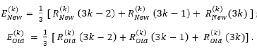
2. Evaluation of the covariance matrix

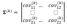
Where

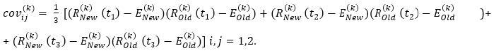
The covariance matrix Σ^(k) is a symmetric one and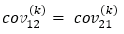

3. Solution of the portfolio problem (5) with parameters Σ^(k) and Σ^(k) with multiple values of λ∈ [0,1]. Each solution gives weights 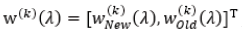and return E^(k)T, W^(k)(λ) as point of the efficient frontier”. Here λ is changed with increment of 0.01 for finding smooth “efficient frontier”.

4. Evaluation of the maximal Excess Sharpe Ratio 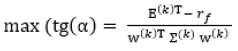and the corresponding weights 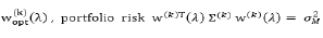and return E^(k)T, W^(k)(λ)=E_M which are stored for final assessments with the BL model.

5. Application of the BL model. Calculation of the “implied asset returns””, according to (7), using E_M and σ²_M from point 4.

6. Estimation of parameters P and Q of the expert views only on the basis of historical data. Analytical relations from [30] are used. The current portfolio contains two assets, “New” and “Old”. Thus, matrix P contains one row for one view with two components P= [α₁ α₂]. The values αi are evaluated according to the difference between the historical mean returns E and the evaluated “implied returns” П. Following [30] 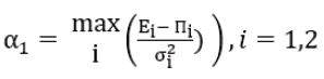is the maximal value of the relative difference (E-П). Respectively, 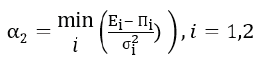is the minimal one. The matrix Q is: Q= (E-П). The matrix Ω is Ω=P(τΣ)P^T

7. Evaluation of the modified asset parameters E_BL and Σ_BL, according to (6)

8. Multiple solution of portfolio problem (51) with E_BL and Σ_BL for λ∈[0,1] and finding the set of solutions W_BLopt(λ^opt)

9. Evaluation of the maximal Excess Sharpe Ratio 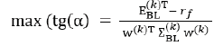and the corresponding weights W^(K)_BLopt(λ) portfolio risk which are stored for assessments with the results from point 4.

10. Increase k for the next sliding period, k=1…7, Figure 4.

The optimal weights of classical and BL models from p.4 and p.9, W_opt(λ^opt) W_BLopt(λ^opt)

Numerical results for the real estate market in Bulgaria

Numerical results are given to illustrate the beginning of evaluations. For k=1, the first three historical values of HPI are: HPI(New)= [0.2 3.9 2.0], HPI(Old)= [1.3 2.3 0.2]. The average returns and covariance are.

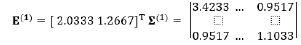
The “efficient frontier” of this portfolio problem for the first sliding period, k=1, is given in Figure 5. The maximal Excess Sharpe Ratio is 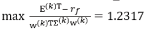where the risk free return for a month is established to γ_f=0.12/12, according to the current policies of the Bulgarian banks. The corresponding weights, giving the maximal Excess Sharpe Return are W_opt^K =[0.1774.8226]^T. The same weights W^K_BLopt(λ) for the BL model are calculated also. The results about obtained for k=1,…,7 are given in Table 1 and the final column presents their mean values. The comparison between the weights of the classical portfolio model, W_opt^(k)(New) and W^(k)_opt(Old), is given in Figure 6, respectively in Figure 7 are the results of weights according to the BL model. Both graphics in Figures 6 & 7 have the same tendencies. The “Old” estates considerably prevail the “New” ones, which gives proves about the potential for investment in “Old” assets. These results are the same, nevertheless of the portfolio problem, which is applied in the evaluations. Comparisons can be made between the characters of curves for the same asset but evaluated with different portfolio model. On Figure 8 are given both graphics for the “New” assets, W_opt^(k)(New) and W^(k)_Blopt(New), evaluated by both classical and BL models. Respectively, Figure 9 makes comparison between the weights of the “Old” assets, W^(k)_BLopt(Old) and W^(k)_BLopt(Old)

Figure 5:Efficient frontier for sliding period k=1.

Figure 6:Portfolio weights W_opt^(k)(New) and W^(k)_opt(Old) evaluated with the classical portfolio model.

Figure 7:Portfolio weights W^(k)_BLopt(New) and W^(k)_BLopt(Old) evaluated with BL portfolio model.

Figure 8:Portfolio weights W_opt^(k)(New) and W^(k)_BLopt(New) evaluated with both portfolio model.

Figure 9:Portfolio weights W^(k)_opt(Old) and W^(k)_BLopt(Old) evaluated with both portfolio model.

Table 1: Portfolio weights with classical and BL models for 9 sliding periods.

Both Figures 8 & 9 prove the same behaviour of the “New” and “Old” estates. The weights of the “New” assets are keeping levels close to zero, while the levels of “Old” are close to 1. These results recommend the investments to be made to “Old” real estates, because they give better return in comparison with the “New” ones. The comparisons with the average values of the assets weights also recommend the “Old” assets. The mean column of Table 1 gives low weights for “New” and high weights for “Old” assets: , 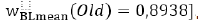. The experiments prove the benefits, which an investor can have, investing in “Old” assets. Here the model does not consider trading taxes, which in real case must be taken in consideration for the final investment decision.

The research presents a way for advanced usage of the portfolio theory. The added value of the paper concerns motivation and illustration of applying sliding mode for portfolio definition and solution. This approach allows being implemented active portfolio management by changing the portfolio decisions on each management step. Additionally, the paper illustrates that the comparison between the portfolio weights can give useful results for the final decision of the investment. The active portfolio management is illustrated by the application of both important portfolio models: the classical Mean-Variance model and the Black-Litterman one. In the paper the subjective views, needed for the BL model has been generated by additional usage of the information, given from the historical data of the asset returns. The subjective views have been generated according to the relative difference between the historically evaluated mean asset returns and the “implied returns”, defined in the BL model. Potential extensions and future researches we find in the possibility to find recommendations about the duration of the historical period, which is applied for the evaluation of the mean asset returns and the corresponding covariation matrix. The length of the history period can be important in finding the length of the investment period, which will give maximal portfolio return. Such analysis currently is not made in this paper.

This work has been supported by project ДH12/10, 20.12.2017 of the Bulgarian National Science fund: Integrated bi-level optimization in information service for portfolio optimization.

1. García-Galicia M, Carsteanu AA, Clempner JB (2019) Continuous-time mean variance portfolio with transaction costs: A proximal approach involving time penalization. International Journal of General Systems 48(2): 91-111.
2. Khan KI, Naqvi SM, Ghafoor MM, Akash RSI (2006) Sustainable portfolio optimization with higher‐order moments of risk. Sustainability 12(5): 1-14.
3. Kolm PN, Tutuncu R, Fabozzi FJ (2014) 60 Years of portfolio optimization: Practical challenges and current trends. European Journal of Operational Research 234(2): 356-371.
4. Malz AM (2011) Financial risk management: Models, history, and institutions. John Wiley & Sons Inc, New Jersey, USA, pp. 752.
5. Schulmerich M, Leporcher YM, Eu CH (2015) Applied asset and risk management. A guide to Modern Portfolio Management and behavior-driven markets. Springer, pp. 476.
6. Markowitz H (1952) Portfolio selection. Journal of Finance 7(1): 77-91.
7. Stoilov T, Stoilova K, Vladimirov M (2019) Saving time in portfolio optimization on financial markets. Intechopen, pp. 330.
8. Sidi SP, Bon AT, Supian S (2017) Modeling of mean-VaR portfolio optimization by risk tolerance when the utility function is quadratic. AIP Conference Proceedings 1827: 1-9.
9. Dowd K (2005) Measuring market risk. (2^nd edn), John Wiley & Sons Inc, New Jersey, USA, pp. 390.
10. Ta VD, Liu CM, Tadesse DA (2020) Portfolio optimization-based stock prediction using long-short term memory network in quantitative trading. Applied Science 10(2): 437.
11. Allaj E (2020) The black-litterman model and views from a reverse optimization procedure: An out-of-sample performance evaluation. J Comput Manag Sci 17: 465-492.
12. Meucci A (2010) The black litterman approach: Original model and extensions. The Encyclopaedia Of Quantitative Finance Pp. 1-17.
13. Chen JM (2018) On exactitude in financial regulation: Value-at-risk, expected shortfall, and expectiles. Journal Risks 6(61): 1-28.
14. Janabi MA (2019) Expert systems in finance. (1^st edn), Taylor Francis group, Abingdon, UK, pp. 1-31.
15. Sharpe W (2010) Adaptive asset allocation policies. Journal Financial Analysts 66(3): 45-49.
16. Bertsimas D, Gupta V, Paschalidis IC (2012) Inverse optimization: A new perspective on the black-litterman model. Journal of Operational Research 60(6): 1389-1403.
17. Chen SD, Lim AEB (2020) A generalized black-litterman model. Journal Operations Research 68(2): 381-410.
18. Harris RDF, Stoja E, Tan L (2017) The dynamic black-litterman approach to asset allocation. European Journal of Operational Research 259(3): 1085-1096.
19. Michaud RO, Esch DN, Michaud RO (2013) Deconstructing black-litterman: How to get the portfolio you already knew you wanted. SSRN Electronic Journal 11(1): 6-20.
20. Stoilov T, Stoilova K, Vladimirov M (2020) Analytical overview and applications of modified black-litterman model for portfolio optimization. Journal Cybernetics and information technologies 20(2): 30-49.
21. Liu C, Shi H, Wu L, Guo M (2020) The short-term and long-term trade-off between risk and return: Chaos vs Journal of Business Economics and Management 21(1): 23-43.
22. Gandomi A, Haider M (2015) Beyond the hype: Big data concepts, methods, and analytics. International Journal of Information Management 35(2): 137-144.
23. Engle R F (1982) Autoregressive conditional heteroscedasticity with estimates of the variance of United Kingdom inflation. Journal Econometrica 50(4): 987-1007.
24. Ranković V, Drenova M, Urosevic B, Jelic R (2016) Mean-uninvariante GARCH VaR portfolio optimization: Actual portfolio approach. Journal Computers & Operations Research 72: 83-92.
25. Sharpe W (1999) Portfolio theory and capital markets. McGraw Hill, New York, USA, pp. 316.
26. Kuester K, Mittnik S, Paolella MS (2006) Value-at-risk prediction: A comparison of alternative strategies. Journal of Financial Econometrics 4(1): 53-89.
27. Black F, Litterman R (1991) Asset allocation: Combining investor views with market equilibrium. The Journal of Fixed Income 1(2): 7-18.
28. Palczewski A, Palczewski J (2019) Black-Litterman model for continuous distributions. European Journal of Operational Research 273(2): 708-720.
29. Idzorek TM (2002) A step-by-step guide to the black-litterman model. Zephyr Associates Inc pp. 1-38.
30. Vladimirov M, Stoilov T, Stoilova K (2017) New formal description of expert views of black-litterman asset allocation model. Journal Cybernetics and Information Technologies 17(4): 87-98.
31. Walters J (2014) Reconstructing the black-litterman model. SSRN Electronic Journal pp. 1-18.
32. Xiao J, Zhu X, Huang C, Yang X, Wen F, et al. (2019) A new approach for stock price analysis and prediction based on SSA and SVM. International Journal of Information Technology & Decision Making 18(1): 287-310.
33. https://www.nsi.bg/en/content/13023/housing-price-statistics.