
- About Us
- Information
-

The Author ensures that the research has been conducted responsibly and ethically with adherence to all relevant regulations. read more..
- For Authors
- For Reviewer
- Manuscript Guidelines
- Membership
- Publication Ethics
-
- Journals
- Reprints
- e-Books
- Videos
- Policies
- Contact Us
 COVID-19
- Submissions


Full Text
Research & Development in Material Science
Measuring Plastic Properties from Sharp Nanoindentation: A Finite-Element Study on the Uniqueness of Inverse Solutions
Fabian Pöhl*
Department of Materials Technology, Ruhr University Bochum, Germany
*Corresponding author: Fabian Pohl, Department of Materials Technology, Ruhr University Bochum, Germany
Submission: December 21, 2017; Published: January 12, 2018

ISSN: 2576-8840Volume3 Issue1
Abstract
Nanoindentation is a non-destructive and simple method to measure important mechanical properties of materials. According to the analysis of Oliver and Pharr e.g. Young's modulus and hardness can determine directly from a measured load-displacement curve [1]. Indirectly the loaddisplacement curve contains the whole stress-strain behavior of the material although it is not directly accessible [2]. Thus the determination of the stress-strain curve from a given load-displacement curve leads to an inverse problem. Several approaches and methods have been developed in order to solve the inverse indentation problem. On the one hand there are approaches based on dimensional analysis [3-7]. On the other hand optimization algorithms were developed. A main problem is that the inverse problem is ill-posed and thus the uniqueness of the inverse solution is often not granted [8,9]. Different material parameter can lead to indistinguishable load-displacement curves. This problem occurs although multiple indenter algorithms are used [10]. In a first step this paper shows for a power-law material behavior (a=Ksn) the problem of non-uniqueness in inverse analysis using an optimization algorithm. In case of a single indenter optimization process the inverse solution is not unique and there is an infinite number of material parameter combinations leading to indistinguishable load-displacement curves. In a second step an energy based mathematical analysis of the problem is introduced, which shows that a mathematical relationship between all possible inverse solutions exists. In order to extract a unique solution a second indenter with a different geometry (different apex angle) is used. The second indenter leads due to changed applied strain field to a second set of inverse solutions and a second mathematical relationship. In case of the two parameters of the power-law the unique solution can be calculated from the two derived equations. This procedure was subsequently checked and verified with finite-element calculations.
Keywords: Indentation; FEM; Stress/strain relationship; Inverse analysis; Uniqueness; Ill-posed problem
Introduction
Figure 1: Schematic illustration of a load-displacement curve including important important indentation parameters.

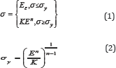
Nanoindentation is often used in mechanical characterization of materials. During an experiment an indenter penetrates normally into the surface of a material. At the same time there are measured simultaneously load P and penetration depth h. The plot of load and indentation depth leads to the load-displacement curve, which is schematically illustrated in Figure 1. The classical analysis of the load-displacement curve according to Oliver and Pharr allows directly the calculation of important mechanical material properties such as hardness and Young's modulus [1].Several research works have shown that a relationship between the load-displacement curve and the stress-strain curve of a material exists but it is not directly accessible [2]. The resulting inverse problem is addressed by dimensional analysis as well as optimization algorithms [3-7]. Optimization algorithms minimize the error between a measured and simulated (Finite-Element- Method) load-displacement curve by adjusting the material parameters within the FE-model. The main problem is related to the non-uniqueness of the inverse solution [8,9]. That means different material parameter combinations can lead to indistinguishable load-displacement curves. This problem has not been solved although multiple indenter algorithms were developed [10]. Within this work a mathematical relationship between possible inverse solutions is derived and used to identify a unique solution of the inverse problem with a dual sharp inverse optimization algorithm and a power-law material behavior. Figure 2 shows a typical stress- strain relationship of a power-law material. According to equation 1, elasticity follows Hooke's law and plasticity power-law hardening. The power-law material model has got two independent variables strength coefficient K and hardening exponent n. The yield stress y is a dependent variable and given by equation 2.
Figure 2: Typical uniaxial stress-strain curve of a power-law material with the material parameters yield stress y, strength coefficient K, strain hardening exponent n, and Young's modulus E.

Inverse Algorithm and FE-model
The general approach of an inverse optimization algorithm is the minimization of the error between a given (measured) and a simulated load-displacement curve by adjusting the material parameters of the FE-model. The minimization process is controlled by optimization/minimization methods and algorithms such as Levenberg-Marquardt, Simplex, SiDoLo or Kalman [11-17]. The algorithms minimize an objective-function, which describes the error between the two curves (e.g. the least squares error of the load), under certain constraints. In this work the Simplex minimization method according to Powell was used to minimize the objective function by adjusting the material parameters of power-law materials using FEM simulations [18,19]. The material parameters of the power-law material are Young's modulus E, strength coefficient K and hardening exponent n (equation 1). The Poisson's ratio has got a minor influence on the curve and is 0.3 for most metals. Hence Poisson's ratio remains constant with 0.3. In order to reduce the number of unknown material parameters the Young's modulus is assumed to be known due to the fact that it can be determined directly from the load-displacement curve with the Oliver and Pharr method [1].
Figure 3: Geometry, mesh and boundary conditions of the FE-model.

FE-simulations were performed using the FE-software ABAQUSr [20]. The FE-model is shown in Figure 3 and based on prior work [21,22]. It is an axisymmetric 2D model with a rigid conical indenter with an half apex angle a. Two conical indenter geometries with different half apex angles are modeled for the dual sharp inverse algorithm (a = 70.3° and 80°). The dimensions of the whole modeled specimen area are 100 x 100 micron. Simulations were carried out displacement-controlled, where the indenter is indented into the specimen with a constant displacement (uy = 1). All other degrees of freedom of the indenter are zero. The sample is supported with symmetry boundary conditions along the symmetry axis and floating supports along the lower edge. The contact between indenter and sample is assumed to be frictionless. The mesh is shown in Figure 3. The area near the contact is meshed finely with quad dominated CAX4R elements with reduced integration and hourglass control. In order to reduce the calculation effort, the fine mesh near the contact region is converted to a coarse mesh of quad CAX4R elements. The transition region between the fine and coarse mesh consists of triangular CAX3 elements. The total element number is 6121.
Results and Discussion
For validation a pseudo-experimental load-displacement curve with known material parameters was simulated. The input material parameters are 2500MPa for strength coefficient K and 0.3 for hardening exponent n. The Young's modulus E and the Poisson’s ratio remain constant with 210GPa and 0.3, respectively. The pseudo-experimental load-displacement curve is used as input data for the single indenter inverse algorithm in order to identify the known input material parameter. Figure 4 shows the pseudoexperimental load-displacement curve as well as three obtained inverse solutions using different start parameters within the optimization procedure. None of the inverse solutions is consistent with the input material parameters, although the load-displacement curves are. That shows clearly the problem of non-uniqueness. Different parameter combinations can lead to indistinguishable load-displacement curves. Thus, all those material parameter combinations are possible inverse solutions.
Figure 4: Indistinguishable inverse solutions for a power-law material behavior with constant Young's modulus E = 210GPa

a.Inverse solutions for an half apex angle of a= 70.3º
b.Inverse solutions for an half apex angle of a= 80º.
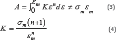
Figure 5 shows the stress-strain curve of two inverse solutions. Although both curves are completely different, they lead to indistinguishable load-displacement curves. In the case of indistinguishable load-displacement curves the same amount of work is done for the elastic and plastic deformation of the material. In uniaxial tensile test the area beneath the stress-strain curve is related to the work that is done during the experiment. Thus, in order to achieve two indistinguishable load-displacement curves with different stress-strain curves the area underneath the stress- strain curves needs to be equal. During the indentation process a strain field is applied by the indenter. In case of a self-similar conical indenter the applied strain field is constant with respect to the indentation depth h. Consequently the area underneath the stress- strain curve needs to be equal until a specific strain (sm) value for all possible inverse solutions. Figure 5 shows the formulated criterion for two obtained inverse solutions of the single indenter algorithm. The elastic part of the stress-strain curve has got a minor influence on the area underneath the curve and the Young's modulus is assumed to be measured directly. Thus, only the plastic part of the stress-strain curve is taken into account.
The area A is given by equation 3. It leads to a simple relationship between the parameters K and n (equation 4). The unknown parameters am and sm in equation 4 can be determined with two inverse solutions or a fit to additional found solutions.
The three obtained inverse solutions lead to am = 829MPa and sm = 0.0581 for the half apex angle a= 70.3° and the considered example. Figure 6 shows the resulting curve. Further found inverse solutions by the optimization algorithm are also given in the plot and are in good agreement with the curve. It shows that possible inverse solutions can be calculated according to equation 5. This equation illustrates the relationship between the two parameters K and n. For an increasing hardening exponent n the strength coefficient K needs to increase in order to achieve indistinguishable load-displacement curves. An increasing hardening exponent causes a drop of the stress-strain curve. This drop can be equalized by an increased strength coefficient leading to the same area beneath the stress-strain curve to the mean strain εm.
Figure 5: Geometry, mesh and boundary conditions of the FE-model.

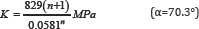
The three obtained inverse solutions lead to am = 829MPa and sm = 0.0581 for the half apex angle a= 70.3° and the considered solutions are illustrated by the curve in Figure 6. The inverse problem has got an infinite number of possible solutions that all result in indistinguishable load-displacement curves. To overcome the problem of non-uniqueness a second conical indenter with a half apex angle of 80° is established, which leads to a different induced strain field in the material and thus to another set of inverse solutions. Figure 4 shows the pseudo-experimental load-displacement curve for the known material parameters and the half apex angle of 80° as well as three different inverse solutions. According to equation 4 the parameters m and "m are determined to 662MPa and 0.0276 for = 80° (equation 6).
Figure 6: Fit of equation 4 to three inverse solutions and further determined inverse solutions that agree with the fit.

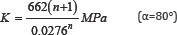
Figure 7: Determination of unique inverse solutions.

The second indenter geometry affords a second curve of possible inverse solutions with am=662 MPa and sm= 0.0276 (equation 6). Due to the different strain field the curve is different from that one of the 70.3° indenter. A unique solution can be determined from the intersection of both curves, which can easily be calculated. Figure 7 shows the two curves and the intersection, which yields to the material parameters K = 2535.7989MPa and n = 0.3007 (input parameter of pseudo-experimental curve: K = 2500MPa and n = 0.3).
Figure 7 shows that in case of two unknown parameters a unique solution can be calculated using two different indenter geometries and equation 4. The identified inverse solution is in very good agreement with the input parameters of the pseudoexperimental load-displacement curve. The error of the strength coefficient K is 1.4 % and that one of the hardening coefficient n is 0.2%.
Summary and Conclusion
The inverse solution of an optimization algorithm is often not unique although multiple indenters are used. In the work presented an inverse optimization algorithm based on the Simplex method was used to identify inverse solutions. For a given half apex angle of a conical indenter a set of inverse solutions can be identified which leads to indistinguishable load-displacement curves. An energy based analysis of the problem shows that a mathematical relationship between possible inverse solutions exists (Equation 4). In the case of the two parameters strength coefficient K and hardening exponent n of the power-law the possible inverse solutions are described by a curve. On the one hand the relationship shows the problem of non-uniqueness. On the other hand it offers the opportunity to determine a unique solution with a second indenter that has got a different half apex angle a. The different half apex angle induces a different applied strain field in the sample. Thus, a different set of inverse solutions and a second inverse solution curve can be obtained. A unique inverse solution can then easily be calculates and is the intersection of both curves. The FEM-investigations show that this procedure is a practical method. A pseudo-experimental load-displacement curve with known material parameters was used for validation. The identified inverse solution was in very good agreement with the pseudo-experimental in-put parameters. The error between the input parameters and the inverse determined is 1.4 % for strength coefficient K and hardening exponent n 0.2 %. The procedure is summarized in Appendix A. Though, the study showed the principal potential to uniquely identify the material parameters from sharp indentation aspects such as the sensitivity and the practical application of the procedure have to be analyzed and discussed.
Appendix
Dual-sharp inverse algorithm:
Measure load-displacement curve with two different selfsimilar indenters (e.g. two different apex angles of a conical indenter)
Determine Young's modulus E according to Oliver and Pharr and assume Poison’s ratio (known for most metals)
Obtain three or more inverse solutions for each indenter geometry with a FEM-coupled optimization algorithm
Fit  to the three inverse solutions of both
Intersection of both solutions is unique inverse solution of the problem (Figure 8).
Figure 8: Fit of equation 4 to three inverse solutions and further determined inverse solutions that agree with the fit.

References
- Oliver WC, Pharr GM (1992) An improved technique for determining hardness and elastic modulus using load and displacement sensing indentation experiments. Journal of Materials Research 7(6): 15641583.
- Tabor D (2000) The hardness of metals, Oxford University Press, Oxford, India.
- Cheng YT, Cheng CM (1998) Scaling approach to conical indentation in elastic-plastic solids with work hardening. Journal of Applied Physics 84: 1284.
- Cheng YT, Cheng CM (1998) Relationships between hardness, elastic modulus, and the work of indentation. Applied Physics Letters 73: 614.
- Tunvisut K, O'Dowd NP, Busso EP (2001) Use of scaling functions to determine mechanical properties of thin coatings from microindentation tests. International Journal of Solids and Structures 38: 335-351.
- Dao M, Chollacoop N, Van-J FK, Venkatesh TA, Suresh S (2001) Computational modeling of the forward and reverse problems in instrumented sharp indentation. Acta Materialia 49(19): 3899-3918.
- Chollacoop N, Dao M, Suresh S (2003) Depth-sensing instrumented indentation with dual sharp indenters. Acta Materialia 51(13): 37133729.
- Cheng YT, Cheng CM (1999) Can stress-strain relationships be obtained from indentation curves using conical and pyramidal indenters? Journal of Materials Research 14(9): 3493-3496.
- Liu L, Ogasawara N, Chiba N, Chen X (2009) Can indentation technique measure unique elastoplastic properties? Journal of Materials Research 24(3): 784-800.
- Chen X, Ogasawara N, Zhao M, Chiba N (2007) Can indentation technique measure unique elastoplastic properties? Journal of the Mechanics and Physics of Solids 55(8): 1618-1660.
- Gamonpilas C, Busso EP (2007) Characterization of elastoplastic properties based on inverse analysis and finite element modeling of two separate indenters. Journal of Engineering Materials and Technology 129(4): 603-608.
- Collin JM, Mauvoisin G, Pilvin P (2010) Materials characterization by instrumented indentation using two different approaches. Materials and Design 31(1): 636-640.
- Bolzon G, Maier G, Panico M (2004) Material model calibration by indentation, imprint mapping and inverse analysis. International Journal of Solids and Structures 41: 2957-2975.
- Nakamura T, Wang T, Sampath S (2000) Determination of properties of graded materials by inverse analysis and instrumented indentation. Acta Materialia 48: 4293-4306.
- Nakamura T, Gu Y (2007) Identification of elastic-plastic anisotropic parameters using instrumented indentation and inverse analysis. Mechanics of Materials 39(4): 340-356.
- Ismail AB, Rachnik M, Mazeran PE, Fafard M, Hug E (2009) Material characterization of blanked parts in the vicinity of the cut edge using nanoindentation technique and inverse analysis. International Journal of Mechanical Sciences 51(11-12): 899-906.
- Kopernik M, Spychalski M, Kurzydlowski KJ, Pietrzyk M (2008) Numerical identification of material model for C-Mn steel using microindentation test. Materials Science and Technology 24(3): 369-375.
- Scpy community (2008) Scipy reference guide: release 0.8.dev.
- Nelder JA, Mead R (1965) A Simplex method for function minimization. Computer Journal 7(4): 308-313.
- (2009) ABAQUS, User's manual v. 6.9, ABAQUS Inc, Providence, USA.
- Pohl F, Huth S, Theisen W (2013) Finite element method-assisted acquisition of the matrix influence on the indentation results of an embedded hard phase. Materials Science and Engineering: A 559(1): 822-828.
- Pohl F, Huth S, Theisen W (2014) Indentation of self-similar indenters: An FEM-assisted energy-based analysis. Journal of the Mechanics and Physics of Solids 66: 32-41.
© 2018 Fabian Pöhl. This is an open access article distributed under the terms of the Creative Commons Attribution License , which permits unrestricted use, distribution, and build upon your work non-commercially.
Editor In Chief


.jpg)


Signup for Newsletter

Quick Links
 Editorial Board Registrations
 Submit your Article
 Refer a Friend
 Advertise With Us
Our Recent Edition

.jpg)


Top Editors


.jpg)


.bmp)
.jpg)
.png)
.jpg)


.jpg)


.png)

.png)


.png)


Financial Support

Sponsors

Latest e-Books

Latest Video

 a Creative Commons Attribution 4.0 International License. Based on a work at www.crimsonpublishers.com.
Best viewed in
a Creative Commons Attribution 4.0 International License. Based on a work at www.crimsonpublishers.com.
Best viewed in