Medium-Term Forecasting of Solar Radiation Using Hybrid Modelling

India’s energy demand could rise to over 3% annually until 2030 due to urbanization and industrialization in the country as per International Energy Agency [1-3]. To meet the rising energy demand as well as to combat pollution, the most easily available and inexhaustible source of energy is solar. However, it is intermittent and diurnal nature. The power output of the solar power plant mainly depends on the incident solar radiation. So, forecasting of power output from solar plants is necessary to maintain the stability of the grid which needs to be balanced for frequency disturbances. The need for solar radiation forecasting is important as the main challenge is to integrate a large number of renewable resources into the conventional energy structure. Accuracy of the forecast of resource data remains essential to a power plant’s efficient operation during its service life. Better forecasting may position renewable energy technologies toward continuous growth and deeper penetration into the global energy mix. The main problem arises due to the intermittent nature of renewable resources, making it difficult to predict its output in advance.

The benefits of renewable energy forecasting are the reduction in the imbalance penalties and charges due to the carrier’s inability of scheduling requirements, savings on cost, the advantage of real-time and day-ahead energy market trading and efficiency in project construction and its operations and maintenance during its service life. The choice of solar forecasting method depends on the timescales involved, which can be classified as given in Table 1. There are several models available for solar radiation forecasting. The model to employ depends on the time horizon of the forecast as well as the use of solar radiation forecasting. The solar radiation forecasting models can be divided into four categories as given in Table 2.

Table 1:Forecast time frames and their applications.

Table 2:Models and features.

For efficient prediction of solar radiation for a shorter duration of intra-day and intra-hour, methods such as time series based models like ARIMA are used. ARIMA model use predictions based on purely past values of solar radiation, but solar irradiance is dependent on various different meteorological factors such as relative humidity, temperature, cloud cover, wind direction, and wind speed. To overcome this shortcoming, nonlinear prediction methods based on Machine Learning (ML) models can be used. ML based models use statistical analysis of past data. They tend to find a relation between a dependent or target variable and one or more independent or predictor variables by training the model. This work focuses on determining the least number of independent variables and using them for the most accurate GHI forecast

There are plenty of machine learning models available to forecast solar radiation. However, for solar radiation forecasting, time series algorithms such as Autoregressive Moving Average (ARMA) and Auto Regressive (AR) are having low forecasting accuracy because of the non-linear characteristics of solar radiation. Solar radiation depends on various meteorological factors such as temperature, wind direction, cloud cover, humidity, and wind speed. Hence, it becomes difficult to find purely temporal correlations and patterns. Artificial Neural Network gives better accuracy than support vector machine and random forest but has challenges such as low robustness to unimportant inputs, complex architecture optimization, enormous training time and need of large dataset. Support vector machine works well for reasonably clean and outlier free datasets. Hence, it is less robust. Also, its accuracy decreases when there is a large amount of dataset.

The random forest model showed the highest accuracy in modelling the daily variability index of solar irradiance due to its ability to capture non-linear relationships between the target variable and the predictor variables [4]. The random forest features cross-validation along with its immunity to irrelevant inputs, and ability of ‘importance capture’. The ‘importance capture’ feature utilizes profile analysis and correlation to select the most appropriate input variables among the predictor variables. For a week ahead forecast, the random forest outperforms the persistent model [5]. The random forest method gives the best accuracy due to the use of randomization of the decision trees. Random forest utilization becomes more critical when the model yields less normalized root mean square error with decreasing time horizon [6]. Random forest is best for its robustness of a large dataset and easy use. It performs well even when some values or data are missing. Due to randomization and averaging of many decision trees, it reduces the effect of any outlier to avoid overfitting and thus increasing the accuracy. Machine learning based models are unable to handle complex non-linear correlations and predicting the solar radiation with low accuracy whereas deep neural networks can handle large amounts of dataset of complex non-linear correlations and also provide better accuracy due to the presence of the neural network.

LSTM based deep neural networks has good feature extraction ability compared to the other conventional machine-learning techniques [7]. The deep neural network models have the ability to endure high noise data from irrelevant data points, the ability to clarify non-linear connections in data, better handling of sequential data, and a memory to store long-term information as well. The LSTM based model was able to outperform support vector machine based model in prediction of short-term hourly solar irradiance for the location of a farm in Canada [8]. LSTM based models can capture 1-D time series data easily and able to generalize the process to fit the model better. It can solve the problems of gradient disappearance and the explosion of the gradient. LSTM model is a deep neural network has feature extraction ability that can endure irrelevant data points and better capture irregularities in the dataset. Forecasting accuracy is the excellent due to presence of memory to store long-term information.

Single models are often insufficient to predict solar radiation with high accuracy due to the non-linear characteristics of solar radiation [2,3]. To improve forecasting performance a hybrid method is better as compared to a single forecasting algorithm [9]. A hybrid model is better at capturing the non-linear characteristic of solar radiation. To develop a hybrid model, the present ensemble models can improve the performance of individual predictors such as decision trees and neural networks. The hybrid model is better than the ensemble model since the hybrid model has the inherent habit of utilizing the unique features from the individual models to provide better results but incase of ensemble model, goes by the method of majority voting selection that yields the less accuracy as compared with hybrid models. Hybrid model is developed using random forest and multilayer perceptron neural network for load forecasting and the results interpret that it outperforms the standalone models such as support vector regression, random forest and multilayer perceptron. The developed hybrid model used the ability of the random forest to segregate major important features and then applied it to the LSTM model to make it simpler, and faster with increased accuracy [10].

The hybrid model was decomposed into linear and nonlinear components. Linear models such as ARIMA (autoregressive integrated moving average) is used to predict the linear component and non-linear component along with the linear residual component is performed by a seasonal multilayer perceptron. This hybridization has been very effective in achieving significant accuracy improvement as compared to the other single models [11]. Using an ensemble of these random forest regression models and LSTM models, a hybrid model can be used to capture both the regression based prediction and time series based prediction of solar radiation. Improved removal of noise and better capture of the series of solar radiation can be ensured by the hybrid model. India is becoming a major hub for solar energy industries as the government is pushing towards renewable energy options to tackle the problem as well as to meet the rising energy demand. The Indian government is making large solar parks such as Bhadla in Rajasthan and looking over floating solar parks as well to meet the requirements. Also, for supporting local industries, the government has launched initiatives for local manufacturing of solar power equipment in the country.

All the government policies and initiatives are launched towards the aim of exploiting the solar energy resources to a greater extent. The effective utilization of solar potential is possible only if there is accurate forecasting of solar radiation. The hybrid model is developed by using random forest and LSTM. The proposed hybrid model has not been explored in India for forecasting solar radiation. There is limited research has been performed on residual prediction based on deep neural network. Feature importance for selecting the most influential parameter has not been utilized in all research for the development of a random forest model. Considering the viewpoints, this work contributes to the development of a random forest regression tree model and then the development of long short term memory. Finally, the hybrid model is constructed with the random forest regression tree and LSTM to forecast the solar radiation in New Delhi, India. The hybrid model uses the least number of features for giving the best accuracy and uses a LSTM model for the residual predictions. This gives the hybrid model an edge over the other individual models giving lower error and better accuracy at prediction.

Data collection

The dataset used in this study is obtained from the National Renewable Energy Laboratory (NREL) [9] which is an open-source dataset easily available. The target of this study is to predict global horizontal irradiance for the location of New Delhi (28.54 °N, 77.19 °E). The data was obtained from NREL for the year 2015 to 2020 on an hourly basis. The dataset obtained included years from 2015 to 2020, months from January to December, days from 1 to 31, hours from 00 i.e., midnight to 23.00 i.e., 11 p.m., minutes from 00 to 59, DHI (Direct Horizontal Irradiance), DNI (Direct Normal Irradiance), GHI (Global Horizontal Irradiance), clearsky DHI (Direct Horizontal Irradiance), clearsky DNI (Direct Normal Irradiance), clearsky GHI (Global Horizontal Irradiance), temperature, pressure, relative humidity and wind speed. The above-mentioned parameters are obtained for New Delhi, India (28.54 °N, 77.19 °E). GHI is the desired output parameter whereas the other parameters year, month, day, hour, temperature, pressure, relative humidity and wind speed are input parameters as predictors.

Random forest: A random forest consists of multiple decision trees which are randomized and averaged over the time period to reduce the error and giving better results compared to a single decision tree.

Decision tree: A Decision tree that resembles an inverted tree like structure. It is a visual representation of consequences and choices that mimics the human level of thinking. It uses topdown strategy such that the root is at the top and it splits further till the end of data. It can be used in both classifications as well as for regression. Here, each internal node of the tree denotes a test on an attribute and every branch represents the outcome of the test. Each leaf or terminal node represents a class label used for classification. A sample decision tree with different terminologies is shown in Figure 1.

Figure 1: Decision tree terminology.

Figure 2: Representation of random forest decision tree.

Figure 3:Working of the random forest algorithm.

The various terminologies associated with a decision tree are root node which is the top node from where the population starts, and all the data is fed here. It gets further split based on various features. A decision node is a node that can be further split based on attribute criteria. Leaf nodes are the end nodes that cannot be further split. These are also called pure nodes. A sub-tree is a small portion of the decision tree. The decision tree algorithm has a major issue of overfitting. In overfitting, the models tend to learn from each training dataset point that leads to model learning from less important data points as well. Therefore, the model accuracy gets decreased. To overcome the above-mentioned challenge, several decision trees are created at the time of training of the dataset. The output is obtained by averaging the output of all these decision trees. This method is called ensemble learning, where these multiple decision trees give better results than a single tree. This makes it more robust to errors as it uses averaging of all the decision trees and not depending on a single decision tree only. Due to averaging multiple decision trees, the effect of any outlier is minimized a large extent thus avoiding any issue of overfitting in the regressor. A schematic and algorithm of random forest decision tree is shown in Figure 2 & 3 respectively.

Long Short-Term Memory (LSTM): LSTM is a deep neural network model that could store sequential data such as time series. This uses multiple memory cells connected in series which use data from the past to predict future data. It is a special recurrent neural network that could solve the major problems of the disappearance of gradients and the explosion of gradients. This happens due to the presence of the gates which use a sigmoid function that generates numbers in the range of 0 and 1 to control the state of the gates. These gates operate based on the information at the time of essential or not necessary. The gates can be adjusted and truncated as per requirement. The schematic of LSTM is shown in Figure 4. There are three types of gates in the cell structure-input gate, forget gate and output gate. The input gate controls new information to be added from current input to selectively replace information removed by forget gate. Memory update aggregates old memory through forget gate and new memory through the input gate.

Figure 4: Schematic of long short-term memory cell.

Forget gate selects information to be removed away from memory and output gate decides the required output from the memory. There are three key variables in the cell structure input (h_t-1) which is the hidden layer at the time (t-1) and x_t which is the feature vector at the time t. The input controls the three gates. The ht is the input of the next cell and is separated from the real output by softmax which is the direct source of output. Mainline or memory namely C_t-1 and C_t are isolated from outside as memory which is attenuated by forget gate and activated based on enter gate control supply size. Output (h_t) which is a hidden layer or plus softmax as the real output.

Data preprocessing

Using raw data in the random forest regression tree, preliminary preprocessing steps are essential to increase accuracy. These steps help to avoid any overfitting and underfitting of the model. One of the preliminary steps is ‘Sample’ which returns a random sample of items from an axis of an object to extract random instances and records from the dataset. Here a sampling of data is from 5AM to 7PM only as there is no sunshine beyond this time period. Feature correlation is used to find correlation of target feature with other features to get their inter-dependence upon on each other. Here the target feature being GHI as given in Table 3. Another preliminary step is featuring importance which assigns a score to all the input features. The scoring is based on the usefulness of predicting the target variable. There are many ways to calculate feature importance scores such as statistical correlation scores, permutation importance scores, etc. It is an important aspect of feature selection and dimensionality reduction. Feature importance for the given input features is shown in the Table 4. At maximum R2 score of 0.9345 the least number of features required are Year, Month, Day, Hour, Temperature and Relative Humidity. This is preferred for the working of the regressor. The available dataset is separated into training data and validation or testing data. It is usually around 70% for training data and 30% for testing purpose.

Table 3:Features correlating with global horizontal irradiance.

Table 4:Feature importance.

Construction of random forest regression tree

Figure 5:Random forest decision tree with a depth of 2.

Random forest regression tree requires these major input parameters for its construction as ‘n_estimators’ which is the number of trees in the forest, by default it is 100. ‘Criterion’ measures the quality of tree split which is “squared_error” here using variance reduction as feature selection criteria. ‘max_depth’ is maximum depth of the tree, which by default is “None” meaning that nodes are expanded until all leaves contain less than min_ samples_split or all leaves are pure. For the best split, the number of features used is ‘max_features’. By default, it is “auto” which means that max_features=n_features. ‘min_weight_fraction_leaf ’ is the minimum weighted fraction of the sum total of weights (of all the input samples) which is essential to be at a leaf node. By default, it is “0.0” which indicates that samples have equal weight and ‘random state’ controls the randomness of the bootstrapping of the samples when used to build trees. The schematic of random forest decision tree is depicted in Figure 5.

Construction of long short-term memory

For the formation of the LSTM model, the input parameters to be set are epoch which is a number of times the model trains over the entire dataset which is 500 here. Learning rate which decides the change in model with respect to error after model weights are updated which is kept as 0.001 here. Neurons which are units within the LSTM cell. It should be kept higher to occupy the non-linearity of the dataset better. The value of neurons is 12. Output neurons are the number of output units which is 1 here for global horizontal irradiance only. The optimizer is the solver for the algorithm which uses the back propagation method. The optimizer used here is ADAM (adaptive moment estimation). It computes learning rates for all the parameters as well as stores the mean and variance of the gradient values.

Construction of hybrid model

The hybrid model is formed by firstly passing the dataset through the random forest regression model where the regressionbased model uses the input features as year, month, day, hour, temperature, relative humidity and sky clearness index. This model is used to estimate the non-linear dependence of global horizontal irradiance. After the prediction of global horizontal irradiance from the model, the residual is calculated as the difference between the predicted and the actual values. The residual is then passed through the LSTM based model to determine the time based linear dependence of GHI. Finally, the prediction of residual from the long short-term model and the GHI prediction from random forest regression model are added up to obtain the final predicted global horizontal irradiance. The workflow of the developed hybrid model is shown in Figure 6.

Figure 6:Flow chart of hybrid model.

The LSTM model was formed with the parameters as given in the Table 5. The model has input layer as LSTM layer with 32 nodes as larger nodes are better able to capture non-linearity as shown by solar radiation. The second layer is hidden layer with 8 nodes and the output layer has one node only for the single output of GHI. All the layers use ReLU (rectified linear unit) as activation function since here solar radiation shows only positive values. The number of parameters come out to be 4,625. The following measurement metrics are used to monitor and measure the performance and accuracy of a model during training as well as during testing.

Table 5:Parameters of LSTM with two hidden layers.

A. Mean Absolute Error (MAE): It is defined as the average of the sum of the absolute difference between the actual values and the predicted values.

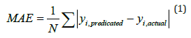
y_{i, predicted} - predicted value of ith data point
y_{i, actual} - actual value of ith data point
N - total number of data points in the data set

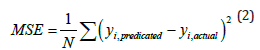
B. Mean Square Error (MSE): It is defined as the average of the sum of the squares of the difference between actual and predicted output values.

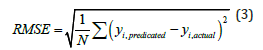
C. Root Mean Square Error (RMSE): It is defined as the square root of the mean square error.

D. Coefficient of determination (R2): It gives an idea about the variance of the data explained by the model. Its value varies between 0 and 1. It is given by the equation:

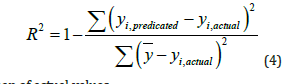
ȳ- mean of actual values
y_{i, predicted} - predicted value of ith data point
y_{i, actual} - actual value of ith data point

The random forest regression model (model 1), LSTM model (model 2) and hybrid model (model 3) were trained and tested for the location of New Delhi (28.54 °N, 77.19 °E). For the final model i.e., hybrid model, the dataset is first passed through a random forest regression model. The residual obtained from the random forest regression model is passed through the LSTM. This is used due to the linearity of the residual with time. The predicted residual from the LSTM model and random forest regression model predictions are combined to obtain the final prediction of GHI.

Performance metrics

The performance metrics of MAE, MSE, RMSE and R₂ are calculated for all three models at New Delhi are represented in Table 6, Table 7 & Table 8 respectively. The random forest regression model was able to perform better as compared to LSTM model and on par with hybrid model as evident from the performance metrics. The hyperparameter ‘max_depth’ decides expansion of decision trees based on splitting of leaves. The proper tuning of the ‘max_ depth’ avoids unnecessary expansion till leaves are pure giving better accuracy. The LSTM model is time series based but solar radiation shows dependence on other atmospheric parameters like temperature, pressure, sky clearance, wind speed, humidity, etc. that diminishes the accuracy as compared to random forest regression model. The hybrid model performance metrics show improved accuracy and decrease in error due to combination of random forest and LSTM model. The combination of time and other atmospheric parameters gives it edge over random forest and LSTM models with increased accuracy.

Table 6:Performance metrics for random forest regression model (Model 1).

Table 7:Performance metrics for long short-term memory model (Model 2).

Table 8:Performance metrics for hybrid model (Model 3).

Comparison of predicted GHI and actual GHI

Figure 7:GHI comparison for actual and three model predictions.

The random forest regression model, LSTM model and hybrid model are trained, tested and validated with the groundbased measurements. Figure 7 shows that the forecasted values from random forest, LSTM and hybrid model validated against the observational values. The random forest regression model performed well other than the high amplitude solar radiation. This occurrence of underfitting of the model is due to unavailability of data points with regard to high value of solar radiation. LSTM model is able to predict very well for high solar irradiance data points but showed deviation for low amplitude solar radiation. The model is unable to capture the periodicity of low amplitude solar radiation but catures well for high amplitude solar radiation which generally happen around afternoon.

Figure 8:Residual comparison between actual and LSTM prediction.

In the hybrid model both the random forest and the LSTM models are used where the LSTM model is to get the residual predictions showing time based dependence of the residual. The predicted residual from the LSTM model and the predicted global horizontal irradiance from the random forest regression model are combined to obtain the final prediction of global horizontal irradiance. The residual prediction performs well at medium residuals but shows large deviation at peaks due to absence of adequate data points for the model to train. It leads to reduction in the accuracy of the hybrid model.

The random forest regression model, long short-term memory model and hybrid model were developed and compared for the prediction of GHI for the location of New Delhi, India (28.54 °N, 77.19 °E). The hourly dataset was from 2015 to 2020 with input features of year, month, day, hour, temperature, pressure, relative humidity, wind speed and sky clearness index.

The hybrid model outperformed the other models as it gives the lowest error in all performance metrics. The hybrid model yields the error value of MAE, MSE, RMSE and R2 as 26.22 W/ m², 1304.45 W/m², 36.11 W/m², and 0.98 respectively. The value of MAE, MSE and RMSE are decreased by 2.42 W/m² & 5.97 W/ m², 256.10 W/m² & 917.85 W/m², and 3.38 W/m² & 11.02 W/m² respectively as compared to random forest and LSTM model. The future research direction of this work is to implement the developed models for different climatic zones in India and evaluate the models performance for various climatic zones.

1. (2022) International Energy Agency (IEA). World Energy Outlook 2022.
2. Seçkin K, Altan A (2019) Recognition model for solar radiation time series based on random forest with feature selection approach. 11^th International Conference on Electrical and Electronics Engineering (ELECO), pp. 8-11.
3. Abuella M, Chowdhury B (2017) Random forest ensemble of support vector regression models for solar power forecasting. IEEE Power & Energy Society Innovative Smart Grid Technologies Conference (ISGT), pp. 2-6.
4. Huang J, Troccoli A, Coppin P (2014) An analytical comparison of four approaches to modelling the daily variability of solar irradiance using meteorological records. Renew Energy 72: 195-202.
5. Lahouar A, Mejri A, Hadj Slama JB (2017) Importance based selection method for day-ahead photovoltaic power forecast using random forests. International Conference on Green Energy Conversion Systems (GECS), pp. 1-7.
6. Benali L, Notton G, Fouilloy A, Voyant C, Dizene R (2019) Solar radiation forecasting using artificial neural network and random forest methods: Application to normal beam, horizontal diffuse and global components. Renew Energy 132: 871-884.
7. Doan VS, Huynh-The T, Kim DS (2020) Underwater acoustic target classification based on dense convolutional neural network. IEEE Geoscience and Remote Sensing Letters 19: 1-5.
8. Alzahrani A, Shamsi P, Dagli C, Ferdowsi M (2017) Solar irradiance forecasting using deep neural networks. Procedia Comput Sci 114: 304-313.
9. Qiu X, Zhang L, Ren Y, Suganthan P, Amaratunga G (2014) Ensemble deep learning for regression and time series forecasting. 2014 IEEE Symposium on Computational Intelligence in Ensemble Learning (CIEL), pp. 0-5.
10. Tharaha S, Rashika K (2017) Hybrid artificial neural network and decision tree algorithm for disease recognition and prediction in human blood cells. International Conference on Innovations in Information, Embedded and Communication Systems, ICIIECS, pp. 1-5.
11. Bahrami M, Khashei M, Amindoust A (2021) A parallel-series hybridization of seasonal intelligent based statistical model for demand forecasting. J Model Manag 17(4): 1126-1143.