Adapting Hartigan & Wong K-Means for the Efficient Clustering of Sets¹

Clustering is a fundamental application in data science. Its goal is to partition data into groups (clusters) in such a way that data in the same cluster are similar to one another, and data in different clusters are dissimilar. The similarity is based on a distance metric that often coincides with the Euclidean distance. K-Means [1,2] is a de facto standard clustering algorithm due to its simplicity and efficiency. Its properties have been thoroughly investigated [3,4]. K-Means, though, normally deals with data points having numerical attributes. Handling data with mixed numerical and categorical attributes or only categorical attributes is difficult [5] and can require introducing a not Euclidean distance function.

Adapting K-Means to clustering data objects which are sets of elementary items, must solve problems similar to the case of categorical attributes. In addition, the need exists to handle sets of different sizes. Recently, an approach to clustering sets was proposed [6] which adapts K-Means and Random Swap [7,8] by using a distance measure that modifies the classical Jaccard or Otsuka-Ochiai cosine distance. The clustering algorithms were then successfully experimented through several benchmark datasets [9]. A different, yet effective, approach was described in [10]. The new approach avoids the problem of finding the meaning of the objects in a cluster, by using the medoid concept [11]. Two algorithms for clustering sets were experimented: K-Medoids [11,12] and a medoid-based version of Parallel Random Swap [8]. With respect to the approach in [6], a distance function among sets was defined which exploits global information about the use of the basic items which compose the sets. The work described in this paper extends the approach described in [10] through an adaptation of K-Means which retains the generality as in [6,10] while providing high computational efficiency and clustering reliability. More in particular, the original contribution is a medoid-based development of the Hartigan & Wong variation of K-Means [13,14], named HWK-Sets, which can work with careful seeding methods [14-18]. Due to the intrinsic good properties of Hartigan & Wong algorithm, HWK-Sets are capable of finding a good clustering solution by few restarts with few iterations.

HWK-Sets are currently implemented in Java by parallel streams [8,19,20] thus ensuring good time efficiency on a multicore machine. The recourse to parallelism is key for scalability, by reducing, in non- trivial datasets, the burden of the 𝑂(𝑁2) computational cost implied by the all-pairwise distance problem which necessarily accompanies the medoids management and the calculation of specific clustering accuracy indexes. The effectiveness of the new clustering algorithm is demonstrated by applying HWKSets to 15 benchmark datasets [6,10]. The experimental results confirm the achievement of reliable clustering solutions with a good computational speedup. The paper is structured as follows. First the background work is briefly reviewed in section II. Then the new algorithm HWK-Sets are detailed in section III, together with some Java implementation issues. The paper continues by illustrating, in section IV, the adopted experimental setup and by reporting the achieved clustering results. Both the clustering accuracy and the computational efficiency are demonstrated. Finally, section V concludes the paper with an indication of on-going and future work.

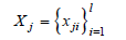
In the following, the main concepts of the work reported in [6,10] are summarized, together with issues of seeding methods and clustering accuracy indexes. A dataset is assumed whose data objects are variable-sized sets of elementary items taken from a vocabulary of size 𝐿 (the problem resolution):

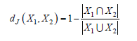
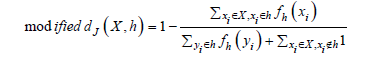
For example, the records of patient diagnoses expressed by ICD-10 [6,21] disease codes can be considered. Clustering such records aims to find groups of similar patients so as to support the estimation of the risk for a patient to develop some future illness due to his/her previous medical history and from correlations to other patients with similar diseases. A key point of the approach in [6] which extends K-Means, named K-Sets, and Random Swap [7,8], named K-Swaps, are the techniques adopted for coping with the mean problem in clusters, which in turn depends on the distance notion among data objects (sets). As a workaround to the difficulty of calculating a mean among sets, a representative data object (centroid) in the form of a histogram is associated with each cluster. The histogram stores its local frequency of use for each item which occurs in the cluster. A histogram contains at most m (e.g., m=20) distinct items. For clusters having more than m items, the first m most frequent items are retained. K-Means partitions data points according to the nearest centroid. A distance measure between a data object (a set) 𝑋 of size 𝑙, and a representative histogram ℎ is proposed which, in a case, modifies the common Jaccard distance between two sets 𝑋₁ and 𝑋₂:

Adaptation is needed because in the case, particularly for large values of L, an intersection between two sets has a few elements in common, the distance measure can lose its meaning. Therefore, for the common items in 𝑋 and ℎ, a weight is used, which is the frequency of the item in the local histogram ℎ:

Similarly, a modified distance notion based on Otsuka-Ochiai cosine can be defined. Assuming, as usual, that the number K of clusters is known, K-Sets initially chooses K representatives in the dataset by a uniform random distribution. Such initial representatives have unitary frequency for each component item. Then the two basic steps of assignment (i.e., partitioning data objects according to the nearest centroid/representative rule) and centroids update (i.e., the new representative of each cluster is established as the new histogram of the items of the data objects which compose the cluster) are iterated. In particular, the objective function cost, i.e., the Sum of Distances to Histogram (𝑆𝐷𝐻) in clusters, is computed after each update step. K-Sets converges when the 𝑆𝐷𝐻 stabilizes, that is the difference between current and previous value of 𝑆𝐷𝐻 is smaller than a numerical tolerance 𝑇𝐻 (e.g., 𝑇𝐻=10−8). The same adaptations apply to K-Swaps which integrates K-Sets as a local refiner of a global centroid configuration that, at each swap iteration, is defined by replacing a randomly chosen representative with a randomly selected data object of the dataset.

Good clustering results are documented in [6], by applying K-Sets (and K-Swaps) to 15 benchmark datasets (𝑆𝑒𝑡𝑠 data in [9]), which all are provided of ground truth information in the form of partition labels for the data objects. Besides the resultant value of the 𝑆𝐷𝐻 cost, the accuracy of a clustering solution was checked by computing the Adjusted Rand Index (𝐴𝑅𝐼) [22] between an emerged solution (partition labels) and the ground truth partition labels. Differently from [6], in [10] a global histogram 𝐻 extracted from the whole dataset is preliminarily built, which associates with each distinct item, in the L vocabulary, its frequency of use in the whole dataset, denoted by f_H(𝑥_𝑖). The global frequency of an item is used as an application-dependent weight which replaces 1 when counting, by exact match, the size of the intersection of two sets; not common items are instead counted as 1. The following is the proposed weighted Jaccard distance:

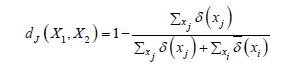
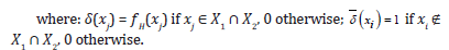
Of course, 1 is the maximal distance between two sets, and 0 the minimal one. If the weights of items evaluate to 1, the distance measure reduces to the standard Jaccard distance. The global histogram was chosen because the occurrence frequency of an item (for example the disease code in a medical application) naturally mirrors a relative importance of the item w.r.t. all the other items. The adoption of the new distance function has some important consequences. First, it enables the distance between any pair of data objects (sets) to be computed, whereas in [6] only the distance from a data object to the local cluster representative histogram can be calculated. Second, the problem of dimensioning the local histogram in [6] is avoided. Third, the new distance permits an exploitation of several seeding methods (see also the next section) including the Maximin [14], K-Means++ [15] and Greedy K-Means++ [16-18] for the initialization of centroids, whereas only the uniform random method is adopted in [6]. Fourth, multiple and expressive clustering indexes can be computed for assessing the accuracy of an achieved clustering solution.

For the abovementioned reasons, the approach in [10] more naturally favors classical K-Means to be adapted for clustering sets. To cope with the mean problem which K-Means demands to solve in the update step, the approach advocated in [10] purposely suggests the use of medoids [11,12]. A medoid always remains a data object of the dataset. It is defined as the particular data object in a cluster, which has minimal sum of the distances to the remaining data objects of the cluster. Here too, the possibility of computing pairwise distances are fundamental. Similarly, to [6], in [10] the Sum of Distances to Medoids (𝑆𝐷𝑀) is assumed as the objective cost to minimize:

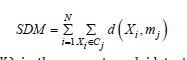
where 𝑚𝑗=𝑛𝑚(𝑋_𝑖) is the nearest medoid to the data object 𝑋_𝑖, that is: 𝑚_𝑗=𝑛𝑚(𝑋_𝑖), 𝑖𝑓 𝑗=𝑎𝑟𝑔𝑚𝑖𝑛_{1≤ℎ≤𝐾} 𝑑(𝑋_𝑖, 𝑚_ℎ). In this paper, the Hartigan & Wong [13,14] variation of K-Means is actually considered (see later in this paper) because of its natural capability of favoring the attainment of better clustering results.

Seeding methods

Let 𝑋_𝑖 be a data object and D(𝑋_𝑖) be the minimal distance of 𝑋_𝑖 to the currently existing L centroids/medoids, 1≤L≤K. All the following methods start by defining the first medoid by a uniform random selection of a data object in the dataset. Each method is then continued until all the K medoids are established.

a. Maximin: the next medoid is defined as a data object of the dataset having maximal D(𝑋_𝑖).
b. K-Means++: the next medoid is defined by a random switch among the data objects of the dataset by first associating to each data object 𝑋_𝑖 the probability of being chosen as:

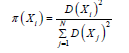
c. Greedy K-Means++: the next medoid is defined by executing S times the K-Means++ procedure and selecting the data object, among the S candidates, which, combined with the L existing medoids, mostly reduces the objective cost. The value 𝑆=⌊2+log 𝐾⌋, suggested in [17], is chosen in the experiments as it represents a trade-off between the improved seeding and the extra computational cost.

Clustering accuracy indexes

In [6] the quality of an achieved clustering solution is evaluated by the (hopefully minimal) 𝑆𝐷𝐻 cost, and the value of the Adjusted Rand Index (𝐴𝑅𝐼) [22] which captures the similarity/ dissimilarity degree between the obtained solution and the ground truth (centroids or partition labels) solution which comes with the benchmark datasets. The 𝐴𝑅𝐼 values are in the continuous interval [0,1] with 1 which mirrors the best similarity, and 0 which expresses the maximal dissimilarity. In this paper, as in [10], besides the values of the Sum of Distances to Medoids 𝑆𝐷𝑀 and 𝐴𝑅𝐼 indexes, the Centroids Index 𝐶𝐼 [23,24] and the Silhouette Index 𝑆𝐼 [8,14,25,26] are also used for assessing the accuracy of a clustering solution. The 𝐶𝐼 value qualifies a solution, by indicating the number of centroids/medoids (or, equivalently, the partition labels of data objects which compose clusters) that were incorrectly determined. A 𝐶𝐼=0 is a precondition for a correct solution. Finally, the 𝑆𝐼 index logically complements the indication of 𝑆𝐷𝑀. Whereas a minimal value of 𝑆𝐷𝑀 mirrors the internal compactness of clusters, a 𝑆𝐼 close to 1 characterizes well-separated clusters. A SI close to 0 denotes a high degree of overlap among the clusters. A SI which tends to -1 indicates incorrect clustering.

As in [8,20], the Java parallel implementation of the proposed clustering algorithm is a key for smoothing the 𝑂(𝑁2) computational cost due to all pairwise distances calculation required, e.g., in the update phase of medoids, as well as in the evaluation of clustering indexes such as the Silhouette Index, and in the implementation of careful seeding methods.

In this work, the Hartigan & Wong variation of K-Means [13,14] was selected because, as shown in [13], it has a lower probability, w.r.t. classical K-Means, to be trapped into a local minimum of the function cost, although with a higher computation cost implied by the data objects exchanges. The Hartigan & Wong’s K-Means was adapted to work with sets and medoids. The operation of the resultant algorithm, named HWK-Sets, is summarized in the Alg. 1. The notation 𝑛𝑚(𝑋_𝑖) indicates the nearest medoid of a data object 𝑋_𝑖.
Algorithm 1. The operation of HWK-Sets
Input: the dataset 𝑋 of 𝑁 data objects, and the number 𝐾 of medoids/clusters
Output: the final 𝐾 medoids and associated clusters/partitions
1.define initial 𝐾 medoids by a seeding method
2.partition the dataset 𝑋 according to the 𝑛𝑚(.) rule
3. set 𝑠=𝑡𝑟𝑢𝑒
4.for each data object 𝑋_𝑖∈𝑋 do
(a)remove 𝑋_𝑖 from its cluster 𝐶_ℎ
(b)update the medoid 𝑚ℎ of modified 𝐶_ℎ
(c)assign 𝑋_𝑖 to cluster 𝐶𝑙 if medoid 𝑚_𝑙=𝑛𝑚(𝑋_𝑖)
(d)update the medoid 𝑚𝑙 of modified cluster 𝐶_𝑙
(e) if 𝑙≠ℎ, set 𝑠 =𝑓𝑎𝑙𝑠𝑒
5. if 𝑠==𝑓𝑎𝑙𝑠𝑒, set 𝑠 =𝑡𝑟𝑢𝑒 and goto step 4
6. evaluate the 𝑆𝐷𝑀 of the final clustering solution.

A critical point in Algorithm 1 is the recurrent update of the medoid during data object exchanges between a source cluster 𝐶_ℎ and a destination cluster 𝐶_𝑙, after having extracted a data object 𝑋_𝑖 from 𝐶_ℎ and added 𝑋𝑖 to 𝐶_𝑙. The new medoid 𝑚_𝑗 of a cluster 𝐶_𝑗 is identified as the data object of 𝐶_𝑗 which has the minimal sum of distances to the remaining data objects of 𝐶_𝑗. Therefore, if 𝑝 is the size of 𝐶_𝑗 and 𝑞 is the maximum size of a data object 𝑋_𝑗∈𝐶_𝑗, the cost for finding the new medoid is 𝑂(𝑝²𝑞²). The overall cost for completing one execution of step 4 of Alg. 1 is 𝑂(𝑁𝑝²𝑞²). Parallelism can be exploited during the computation of a new medoid, when all the pairwise distances among the data objects within a cluster need to be generated. Such a cost could be minimized by building and keeping the matrix of all the pairwise distances in the dataset. However, considering the unacceptable memory cost of such a matrix in large datasets, the HWK-Sets implementation purposely maintains, in each data object, the sum of the distances to all the remaining data objects of the same cluster.

Due to the stochastic initialization of the medoids in HWKSets, implied by many seeding methods, the algorithm needs to be repeated a certain number of times and the emerging best solution, with minimal SDM, minimal (hopefully 0) Centroid Index CI, and maximal (hopefully 1) Adjusted Rand Index ARI and Silhouette Index SI, detected and persisted.

Implementation issues

An efficient implementation of HWK-Sets was achieved on top of Java parallel streams [8,19,20], which rest on the fork/ join mechanism and a lock-free multi-threaded organization. The dataset is split into multiple segments, and separate threads are spawned to process the data objects of segments. Finally, the partial results produced by working threads are combined to generate the result. The operations to accomplish on the data objects are conveniently expressed in a functional way by lambda expressions, with the semantic constraint to avoid, in the lambda expressions, any access and modification to shared data which would cause data inconsistency problems. The basic rationale of the implementation is to support an incremental strategy of the update operations required during data object exchanges (steps from 4(a) to 4(d) in Algorithm 1). First the initial partitions/clusters are built (see step 2 of Algorithm 1). After that, for each data object, the total sum of distances to the remaining objects of the same cluster is computed and held in the data object. The provision aims to reduce the computations required during data exchanges in the steps from 4(a) to 4(d) of Algorithm 1, that is local updates to clusters, including the distance sums maintained in the data objects. All of this is a key for improving the calculation of new medoids in the two clusters involved in data exchange.

Algorithm 2 details the partition step 2 of Algorithm 1, which creates the initial clusters.

Algorithm 2. Initial partitioning (step 2 of Algorithm 1).
Stream p_stream=Stream.of(dataset);
if( PARALLEL ) p_stream=p_stream.parallel();
p_stream
.map( p -> {
double md=Double.MAX_VALUE;
for( int k=0; k< K; ++k ) {
double d=p.distance(medoids[k]);
if( d < md ) {
md=d; p.setCID(k);
}
}
clusters[p.getCID()].add(p);
return p; } )
.forEach( p->{} );

A critical point in the Algorithm 2 is that each data object can be processed in parallel. Therefore, to avoid inconsistencies, each data object 𝑝 only modifies itself (its medoid identifier CID) in the 𝑚𝑎𝑝() method. However, managing cluster partitions (lists) also requires care against simultaneous modifications issued by multiple threads which process data objects belonging to the same cluster. This problem was solved by realizing partition clusters as 𝐶𝑜𝑛𝑐𝑢𝑟𝑟𝑒𝑛𝑡𝐿𝑖𝑛𝑘𝑒𝑑𝑄𝑢𝑒𝑢𝑒 s which are totally lock-free and safe against simultaneous access by multiple threads. The terminal operation 𝑓𝑜𝑟𝐸𝑎𝑐ℎ() in Algorithm 2, serves only to trigger the execution of the intermediate 𝑚𝑎𝑝() operations. Following the initial formation of clusters, the total sum of the distances of each data object 𝑝 to the remaining objects of the same cluster is computed and stored in 𝑝 as shown in Algorithm 3. Algorithm 4 shows the computation of the new medoid of the cluster ℎ from which the data object 𝑋_𝑖 is extracted (see step 4(a) in Algorithm 1). From all the remaining data objects in cluster ℎ, the distance to 𝑋_𝑖 is subtracted. Similar operations are executed for defining the new medoid of the cluster 𝐶_𝑙 to which the object 𝑋_𝑖 is added (step 4(d) of Algorithm 1).

Algorithm 3. The total sum of distances of data objects for( int h=0; h< K; ++h ) {
Stream cStream=clusters[h].stream();
if( PARALLEL ) cStream=cStream.parallel();
final int H=h; //turn h into an effectively final variable cStream
.map( p->{
double sum=0D;
for( DataObject q: clusters[H] ) {
if( q!=p ) sum=sum+p.distance(q);
}
p.setDist(sum);
return p;
})
.forEach( p->{} );
}
Algorithm 4. Medoid computation of step 4(b) of Algorithm 1.
Stream cStream=clusters[h].stream();
if( PARALLEL ) cStream=cStream.parallel();
neutral.setDist( Double.MAX_VALUE );
final int I=i;
DataObject best=cStream
.map( p->{
p.setDist( p.getDist()-p.distance( dataset[I] ) );
return p;
})
.reduce( neutral, //neutral data object for comparisons (p1,p2)->
{ if( p1.getDist()< p2.getDist() ) return p1;
return p2; }
);
medoids[h]=new DataObject( best );
medoids[h].setN( clusters[h].size() );

The incremental update operations during the data exchanges can ensure a good execution performance (see later in this paper), although the intrinsic sequential behavior of Algorithm 1.

HWK-Sets were applied to 15 synthetic datasets which were experimented in [6,10] and which are available from [9]. The benchmark datasets are reported in Table 1. All the datasets are composed of N=1200 data objects and are characterized by the particular size 𝐿 of the vocabulary of elementary items, the number 𝐾 of clusters, the overlapping degree (the 𝑜 percentage) and the type 𝑡 of clusters. The type 𝑡 can specify equally sized clusters (𝑡=1) or various cases of unbalanced clusters. The design parameters are recalled in the name of the dataset: 𝑑𝑎𝑡𝑎_𝑁_𝐿_𝐾_𝑜_𝑡 (see Table 1). Particular combinations of the parameter values can make challenging the clustering process. Ground truth partition labels are provided for each benchmark dataset, which are useful for checking the clustering accuracy by the 𝐴𝑅𝐼 index and the 𝐶𝐼 Centroid Index [23,24]. All the execution experiments were carried out on a Win11 Pro, Dell XPS 8940, Intel i7-10700 (8 physical cores), CPU@2.90 GHz, 32GB Ram, Java 17.

Table 1:Synthetic datasets for clustering sets.

Experimental results

Due to its intrinsic behavior based on data exchanges among clusters, Hartigan & Wong’s K-Means (see also [13]) tends more naturally to evolve the centroids toward their optimal positions. Therefore, few repetitions of HWK-Sets are in general expected to be required for generating a good clustering solution, particularly when a careful seeding method is employed. Table 2 shows some preliminary results related to 𝑅=100 repetitions of HWK-Sets applied to the challenging thirteenth dataset in Table 1, which has the maximum number of clusters to fulfill, separately under the uniform random (UNIF) and the Greedy K-Means++ (GKM++) seeding. The average values of the 𝑆𝐷𝑀 (𝑎𝑆𝐷𝑀), 𝐴𝑅𝐼 (𝑎𝐴𝑅𝐼) and 𝐶𝐼 (𝑎𝐶𝐼) are reported, together with the Success Rate (𝑆𝑅), that is the number of experiments among the 𝑅 which terminate with a 𝐶𝐼=0, the average number of iterations (𝑎𝐼𝑇) executed per repetition/ run, and the parallel elapsed time (𝑃𝐸𝑇) in sec. The benefits of careful seeding emerge from Table 2. On average, GKM++ requires fewer iterations to HWK-Sets and ensures better values of the clustering indexes. Table 3 is an update of Table 2 when 𝑅=20 repetitions are used. The superior character of GKM++ w.r.t. UNIF is confirmed. Table 4 collects the values of the best solution which emerged among the 𝑅=20 repetitions, under the UNIF and GKM++ seeding methods, that is the solution with minimal 𝑆𝐷𝑀, and the corresponding values of the 𝐴𝑅𝐼, 𝐶𝐼 and 𝑆𝐼. As one can see from Table 4, HWK-Sets was able to find a very good solution with the two seeding methods, although GKM++ ensures greater accuracy. It should be noted that the result 𝐶𝐼=0 always occurs at the minimum of 𝑆𝐷𝑀, and that the success rate observed with GKM++ (see Table 3) is higher than that of UNIF.

Table 2:Average results of HWK-Sets applied to the dataset 13 of Table 1 under different seeding methods-R=100 repetitions.

Table 3:Average results of HWK-Sets applied to the dataset 13 of Table 1 under different seeding methods-R=20 repetitions.

Table 4:Best results of HWK-Sets applied to the dataset 13 of Table 1 under different seeding methods-R=20 repetitions.

Table 5 reports the best solution clustering data (minimal 𝑆𝐷𝑀 and corresponding values of 𝐴𝑅𝐼, 𝐶𝐼 and 𝑆𝐼) observed when HWL-Sets is applied, with GKM++ seeding and 𝑅=20 repetitions, to all the datasets of Table 1. The high quality of the clustering solutions is confirmed by the high value of the 𝐴𝑅𝐼 index (not less than 0.98) and the 𝐶𝐼 which was found always to be 0. The Silhouette Index SI, in addition, closely mirrors the overlapping degree among the clusters, paired with the number of clusters. For a comparison with the results reported in [6], the values in Table 5 can be averaged respectively according to the number of clusters 𝐾 which varies in {4,8,16,32}, the vocabulary size 𝐿 which varies in {100,200,400,800}, the percentage of overlapping degree 𝑜 which varies in {0,5,10,20,40}, and, finally, the type of cluster unbalance 𝑡 which ranges in [1..5]. For practical reasons, only the average 𝐴𝑅𝐼 values, which reveal the clustering accuracy, are compared. Indeed, in [6] the 𝐶𝐼 and the 𝑆𝐼 indexes were not computed. Moreover, the Sum of Distances to Histogram 𝑆𝐷𝐻 is not directly comparable to the 𝑆𝐷𝑀 values collected by HWK-Sets, because in [6] the adjusted Cosine distance is used whereas, in this paper and in [10], local histograms are not adopted and the modified Jaccard distance is employed. Finally, only the results in [6] obtained with the high precise and fast K-Swaps algorithm (applied with 300 iterations) are used for comparison. Results are in the [Tables 6-9]. Last column is the average 𝐴𝑅𝐼 of the values in the corresponding row. As one can see from Tables 6-9, even with 𝑅=20 repetitions of HWKSets the accuracy is almost identical to that achieved with K-Swaps in [6].

Table 5:Best solution found by HWK-Sets when applied to all the datasets in Table 1 under GKM++ and R=20 repetitions.

Table 6:ARI vs. K.

Table 7:ARI vs. L.

Table 8:ARI vs. o.

Table 9:ARI vs. t.

Execution performance

HWK-Sets can be executed in parallel or sequential mode. This is regulated by the PARALLEL parameter whose value 𝑡𝑟𝑢𝑒 enables the use of parallel streams with fork/join [8,19]. It should be noted that, in either execution mode, the algorithm executes exactly the same operations as required by the Amdahl law. To figure out the execution performance which parallel streams can provide to HWK-Sets, the clustering algorithm with GKM++ seeding and 𝑅=20 repetitions, was applied 10 times to the dataset 13 in Table 1, and the elapsed time in the parallel (PET) and the sequential mode (SET) observed. Table 10 shows the measured times in sec. From the values in the Table 10, the average SET (aSET) and average PET (aPET) were derived to be: aSET=50.6, aPET=11.5, with a speedup of:

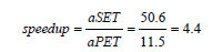
Table 10:Parallel and Sequential Elapsed Time of 10 executions of HWK-Sets applied to dataset 13 of Table 1, with GKM++ and R=20 repetitions (8 physical cores).

The speedup value mirrors the intrinsic sequential behavior which exists in the Alg. 1. Parallelism is exploited in the medoids update operations in the steps 4(b) and 4(d), by working, through parallel streams, on the data objects of the two clusters involved in the exchange operations of an object 𝑋_𝑖. On the other hand, the size of the clusters is relatively small due to the benchmark datasets which have only 1200 data objects.

Clustering sets is difficult because objects are not points with a given dimension of numerical coordinates, and the similarity can’t be expressed by the usual Euclidean distance. In addition, the use of a clustering algorithm like K-Means [1,2] faces the problem of defining the mean of the data objects which populate a cluster. This paper proposes HWK-Sets which extends the Hartigan & Wong’s K-Means algorithm [13] for clustering sets [6]. HWK-Sets, similarly to the work reported in [10], depends on a distance function among sets which, in a case, modifies the Jaccard distance by taking into account application-sensitive information as the global frequency of use of the elementary items which compose the sets. Differently from [6], HWK-Sets can exploit several stochastic seeding methods and the quality of a clustering solution can be assessed by many clustering indexes. The mean problem is tackled by establishing the medoid [11,12] data object as the representative of each cluster. Moreover, HWK-Sets has a natural parallel implementation in Java based on streams [8,19,20] which improve the execution performance. HWK-Sets was successfully applied to the 15 benchmark datasets used in [6,10], thus confirming, with few runs and for each run with few iterations, the same accuracy of the fastest K-Swaps algorithm described in [6]. The prosecution of the work will address the following points. First, to integrate into HWKSets an approach for the incremental evaluation, as in [26], of the Silhouette Coefficients (SC) of data objects, so as to constrain the exchange of a data object from a cluster to another to the condition that the individual SC gets increased. The technique should improve the identification of well-separated clusters. Second, to port the implementation of HWK-Sets on top of the Parallel Theatre actors’ system [27] which favors a better exploitation of the computing resources of a modern multi-core machines. Third, to apply HWKSets to the clustering of pure categorical datasets.

1. Lloyd SP (1982) Least squares quantization in PCM. IEEE Transactions on Information Theory 28(2): 129-137.
2. Jain AK (2010) Data clustering: 50 years beyond K-means. Pattern Recognition Letters 31(8): 651-666.
3. Fränti P, Sieranoja S (2018) K-means properties on six clustering benchmark datasets. Applied Intelligence 48(12): 4743-4759.
4. Fränti P, Sieranoja S (2019) How much can K-means be improved by using better initialization and repeats? Pattern Recognition 93: 95-112.
5. Hautamäki V, Pöllänen A, Kinnunen T, Lee KA, Li H, et al. (2014) A comparison of categorical attribute data clustering methods. Structural, Syntactic, and Statistical Pattern Recognition: Joint IAPR International Workshop, S+ SSPR Proceedings, Springer Joensuu, Finland, pp. 53-62.
6. Rezaei M, Fränti P (2023) K-sets and K-swaps algorithms for clustering sets. Pattern Recognition 139: 109454.
7. Fränti P (2018) Efficiency of random swap clustering. Journal of Big Data 5(1): 1-29.
8. Nigro L, Cicirelli F, Fränti P (2023) Parallel random swap: A reliable and efficient clustering algorithm in Java. Simulation Modelling Practice and Theory 124: 102712.
9. (2023) Repository of datasets.
10. Nigro L, Fränti P (2023) Two medoid-based algorithms for clustering Sets. Algorithms 16(7): 349.
11. Kaufman L, Rousseeuw PJ (1987) Clustering by means of medoids. Statistical Data Analysis Based on the L1-Norm and Related Methods.
12. Park HS, Jun CH (2009) A simple and fast algorithm for K-medoids clustering. Expert systems with applications 36(2): 3336-3341.
13. Slonim N, Aharoni E, Crammer K (2013) Hartigan’s K-means versus Lloyd’s k-means-is it time for a change? In IJCAI, pp. 1677-1684.
14. Vouros A, Langdell S, Croucher M, Vasilaki E (2021) An empirical comparison between stochastic and deterministic centroid initialization for K-means Machine Learning 110: 1975-2003.
15. Arthur D, Vassilvitskii S (2007) K-Means++: the advantages of careful seeding. Proceedings of the ACM- SIAM Symposium on Discrete Algorithms, pp. 1027-1035.
16. Celebi ME, Kingravi HA, Vela PA (2013) A comparative study of efficient initialization methods for the K-means clustering algorithm. Expert systems with applications 40(1): 200-210.
17. Baldassi C (2020) Recombinator-k-means: A population-based algorithm that exploits k-means++ for recombination. arXiv:1905.00531v3, Artificial Intelligence Lab, Institute for Data Science and Analytics, Bocconi University, via Sarfatti 25, 20135 Milan, Italy.
18. Baldassi C (2022) Recombinator-k-means: An evolutionary algorithm that exploits k-means++ for recombination. IEEE Transactions on Evolutionary Computation 26(5): 991-1003.
19. Urma RG, Fusco M, Mycroft A (2019) Modern Java in Action. Manning, Shelter Island, New York, USA.
20. Nigro L (2022) Performance of parallel K-means algorithms in Java. Algorithms 15(4): 117.
21. (2019) ICD-10 Version.
22. Rezaei M, Fränti P (2016) Set matching measures for external cluster validity. IEEE Transactions on Knowledge and Data Engineering 28(8): 2173-2186.
23. Fränti P, Rezaei M, Zhao Q (2014) Centroid index: cluster level similarity measure. Pattern Recognition 47(9): 3034-3045.
24. Fränti P, Rezaei M (2016) Generalized centroid index to different clustering models. Joint Int. Workshop on Structural, Syntactic, and Statistical Pattern Recognition, 10029, LNCS, Merida, Mexico, pp. 285-296.
25. Rousseeuw PJ (1987) Silhouettes: A graphical aid to the interpretation and validation of cluster analysis. Journal of Computational and Applied Mathematics 20: 53-65.
26. Bagirov AM, Aliguliyev RM, Sultanova N (2023) Finding compact and well separated clusters: Clustering using silhouette coefficients. Pattern Recognition 135: 109144.
27. Nigro L (2021) Parallel theatre: an actor framework in Java for high performance computing. Simulation Modelling Practice and Theory 106: 102189.