Meta-Analysis of a Very Low Proportion Through Adjusted Wald Confidence Intervals

Meta-analysis, which is a statistical technique for combining the findings from independent studies, can be used in many fields of research, having high importance in clinical and epidemiological contexts [1]. The meta-analysis for one effect size provides a precise estimate effect and increase statistical power by combining results of independent studies. In the meta-analysis, the pooled effect size measure (θˆ) could be seen as a linear combination of several effect sizes studies

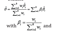
where w_i is the weight of the effect size of study i. There are two well-known models of performing meta-analysis that we will consider in this study: fixed-effect and random-effects models. The model of fixed effect is adequate when homogeneity in effect sizes exists between studies. According to the inverse variance (IV) method, is the sampling error variance associated to the ith study. In the presence of heterogeneity between studies, it was usually used the random-effects model, which incorporates the within-study variance and the between-studies variance . Under random-effects model context, there are closed form and iterative methods to estimate the between-study variance, in [1] can be found 16 distinct methods. However, the most popular procedure to estimate the betweenstudy variance is the Der Simonian and Laird (DL) method [2], and it is the default option in several meta-analysis software’s. Here, we focus in the most popular meta-analysis methods, resuming the methods by some differentiator features (Table 1). For the random-effects models the methods described in Table 1 use the estimator of between-study variance/ heterogeneity which can assume distinct options. The DL estimator of τ is given by and Q the Cochran’s Q-statistic Paule.

and Mandel (PM) method [3] is similar to DL method with other τˆ . The PM approach provide an iterative process to compute τˆ , a disadvantage of this iterative estimator is that they depend on the choice of maximization method and the convergence could fail. There are other similar alternative methods (with the above mentioned), for example, the method proposed by Sidik & Jonkman SJ [4] is similar to Hartung and Knapp (HK) method with other τ estimator proposal. The DL estimator of between-study variance appears to perform adequately. However, several simulation studies have been proposed to compare distinct meta-analysis procedure and there are several specific conclusions. According [5], the most recent review, PM method appears to have a more favorable profile among other estimators of between-study variance. The traditional meta-analysis assumes the approximate normal within-study model, which may not a good option in the context of rare events. The rare events topic is widely discussed in the literature. Several approaches have been proposed for the meta-analysis of two treatment groups with rare events (see, for example, the Pepto’s method [6]; approaches based on Poisson random-effects model [6]; approaches based on generalized linear mixed model [7]; unweighted methods [8]; and a review of methods for the metaanalysis of incidence of rare events [9]). And Sweeting et al. [10]. show that the continuity correction is not an adequate option in meta-analysis of rare events.

Table 1:Several meta-analysis methods and principal features. one within-study variance estimator.

Here, we focus on the meta-analysis of one proportion. The meta-analysis of proportions is usually carried out via three well known methods: the classic Wald method (Wald-0) [11], the logit transform, and the Freeman-Tukey double arcsine transform methods [3]. The inverse of the Freeman-Tukey double arcsine transformation method is preferred over the logit and classic Wald methods [3], in particular for large or small proportions. The binomial-normal model was proposed in the context of exact within study likelihood models and was suggested for the meta-analysis of one proportion with rare events [11,12] (method described in Table 1 as GLMM method). In the meta-analysis of one proportion p, the Wald method can be seen as a linear combination of k estimated proportions . We think, there is room for improvement in the case of the estimation of the pooled proportion for a single treatment group in a rare events context. In this paper, we discuss an adapted application of the adjusted Wald method for a linear combination of proportion in the meta-analysis of quasi extreme proportion p≤0.05.

Adjusted wald estimate

Consider k independent binomial studies, , and denote by p_i the proportion of success (the effect size under study) and by n_i the size of the ith study. In each study, an adjusted estimate of the effect size , denoted by i p , is calculated using the parametric family of shrinkage estimators [4,10]

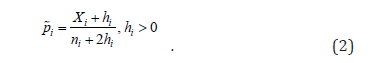
Depending on the particular hi parameter chosen, several different estimators can be considered (Table 2). When, for example, h_i = 0, we have the maximum likelihood estimator (MLE) of p_i. A linear combination of binomial proportions is defined as ,

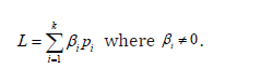
Using equation 2, we have , which converges asymptotically in distribution to a normal distribution,

with the variance of the L estimator. There are several variants of the Wald method to estimate the linear combinations of binomial proportions [1,2,10], where the approximate confidence interval CI for L could be, in general, given by q

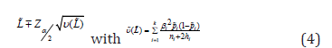
Table 2:Table 2. Parameters hi for the classic and adjusted Wald CI methods in the estimation of p_i based on the parametric family The sets associated to the indicator functions Ai 1  are given by , and .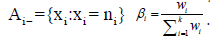

Table 2 shows five variants of the Wald method, identified by Wald-i, i∈ {0,1,2,3,4}. In Wald-3 and -4 variants in the h_i expression assumes different values depending on the CI limits: for the lower bound 1_Ai+ = 0 and for the upper bound 1_Ai− = 0 (Table 2). On the one hand, the parameter hi depends on βi in the Wald-4 variant (Table 2), i.e. hi depends on w_i, it is necessary to adapt this adjusted Wald procedure to perform meta-analysis. On the other hand, 1_Ai++1_Ai− could take different values depending on the CI limits, we use B_i = {x_i:x_i = n_i∨x_i = 0} in the estimation of the weight wi. So, for meta-analysis Wald-4 variant, the parameter h_i is chosen to be in the estimation of the weight w_i. There are several approximate adjusted Wald confidence intervals (CIs) for the meta-analysis of one proportion. The approach developed here uses a parametric family of shrinkage estimators for estimating the proportions. Two popular statistical models, the fixed-effect model and the random-effects model, are used and discussed in this paper. Under the fixed-effect model, we assume that all studies in the analysis share the same true effect size p, that is, p₁ = ··· = p_k = p, and the adjusted pooled prevalence is given by

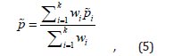
where w_i is the adjusted weight assigned to each study, where w_i is the adjusted weight assigned to each study (as previously defined, is unknown). Taking into account the inverse variance method, the weight could be estimated by

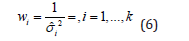
where 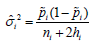is a within-study adjusted variance estimate. Note that the weights and the estimated weights are interchangeably denoted by wi in this paper. Under the randomeffects model, we assume that the true effect size could vary from study to study, in addition to the sample error (σ_i²) there is variability between studies (τ²). The pooled prevalence is also given by equation 5, the weight assigned to each study could assume several estimates (Table 1).

Transformation methods

The meta-analysis can also be performed by using a linear combination of transformed proportions, where several metaanalysis methods were applied to the transformed sampling proportion. The approach based on the transformation of one proportion was typically applied to overcome two well-known constraints: the support range between 0 and 1 and a nonhomogeneous variance. The most common transformations of one proportion are the logit and Prematurely double arcsine transformations,

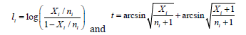
respectively, which are the ones we will consider in this paper when performing the comparison between the meta-analyses of one proportion. The meta-analysis will be applied under the transformed effect size (proportion) and the back transformations will be applied to obtain the result to estimate the overall proportion. In the meta-analysis of proportion, the Freeman-Tukey double arcsine approach it was taken as default and was point as the preferred transformation [13]. The main working example of this work is the prevalence meta-analysis of a multiresistant Staphylococcus aureus bacteria, carrying the new mecC gene [8]. This metanalysis included 25 studies and the sample sizes ni range between 6 and 56382, there are six studies with no occurrences of mecC gene in Staphylococcus aureus. And there are strong and significant heterogeneity between studies included in this metaanalysis.

Monte carlo simulations

To perform the simulation studies, we closely follow the order of magnitude of the prevalence for the mecC gene in Staphylococcus aureus [8]. The overall estimated prevalence of the mecC gene was obtained through the Freeman-Tukey double arcsine transformation method and the random-effects model. The pooled prevalence obtained through this method was 0.009 (95% CI = 0.005-0.013). A simulation study was carried out to compare the adjusted Wald CIs amongst themselves and with those obtained by the best-known transformations: logit and Freeman-Tukey double arcsine. We used a Monte Carlo simulation to compare the performance of the different CIs. The performance of each CI was analysed under the random-effects and fixed-effect models [14], although we are mainly interested in discussing the results arising from the random-effects model. We discuss the meta-analysis methods for the proportion effect size (e.g. prevalence, incidence), pointing our interest in rare events that take into account the practical problem of estimating one low or very low prevalence/incidence. Motivated by the small prevalence values and the simulation scenario proposed in [15], we assume three distinct small proportions, 0.05,0.01 and 0.001 when using the fixed-effect model, and three normal distributions with mean and deviation (0.05, 0.005), (0.01, 0.001) and (0.001, 0.0001), respectively, when using the random-effects model under the heterogeneity hypothesis. The simulation was designed to produce 200000 pooled proportions for each scenario. The proposed comparison is based on four measures computed for each scenario: mean; bias=mean-p; mean square error (MSE)=variance+ bias2 and coverage probability (CP) = (number of CIs containing p)/200000. The used significance level (nominal value) is α=0.05.

We assessed the performance of each CI using the fixed-effect and random-effects models. We studied the performance of the methods considering 25 studies for small proportions. Since in the main working example, the meta-analysis of the prevalence of the mecC Methicillin-resistant Staphylococcus aureus (MRSA), there was a total of 25 studies with rare events. Table 3-5 show the performance of the seven estimation methods under analysis for the fixed-effect and random-effects models, in the context of small proportions (0.05,0.01 and 0.001) for k = 25 using ˆτ as DL or PM estimator, respectively. DL estimator has chosen to analyze the performance in meta-analysis of this small proportion due its popularity and PM estimator was chosen since it was indicated as having overall good performance [16]. Taking into account the proportions under study and the most used methods (IV and DL method with Wald-0, Logit or double arcsine approach) to perform the overall interval estimation, the variant-3 or variant-4 of the adjusted Wald method is a credible competitor to traditional methods, in some cases with the best coverage probability (Tables 3 & 4). By using PM estimator, the results provided by the methods Wald-3 and Wald-4 exhibited comparatively with the other methods, better results, yet no pattern was identified between the different results (Table 5). We also applied our simulation procedure to other methods proposed in the cited literature (Table 1). For the scenario under study, p∈ {0.05,0.01,0.001}, we obtain other methods with good accuracy (Table 6). We sort the results by the coverage probability - CP (Table 6 or complete tables in the supplementary material) and we observe unweighted/double arcsine as the best coverage probability method for p=0.05 and p=0.01 and DL/Wald-3 method for p=0.001 [17-19].

Table 3:Results of the evaluation measures for the CIs obtained through the different approaches with IV method, for k=25, small prevalence with the fixed-effect model. MSE-mean squared error; CP-coverage probability. Good CP results are pointed out in bold.

Table 4:Results of the evaluation measures for the CIs obtained through the different approaches with DL method, for k=25, small prevalence with the random-effects model. MSE-mean squared error; CP - coverage probability. Good CP results are pointed out in bold.

Table 5:Results of the evaluation measures for the CIs obtained through the different approaches with PM method, for k=25, small prevalence with the random-effects model. MSE - mean squared error; CP - coverage probability. Good CP results are pointed out in bold.

Table 6:Methods with the first five best coverage probabilities for the CIs, considering for k=25 and three small prevalence’s in the random-effects model context.

Table 7:Results by method for the mecC MRSA example [8], in the context of random-effects model. The used method vs the alternatives with best coverage probability.

The meta-analysis for the mecC MRSA example was performed with the random effects model due the presence of significant heterogeneity. Motivated by our simulation study, we re-estimated the pooled prevalence using the alternatives with best coverage probability [20,21]. The estimated prevalence’s, obtained by the methods with better performance in probability of coverage, are lower than that presented by [8], (approximately 0.004 vs 0.009, Table 7). Although the estimated prevalence has halved, the updated results did not show significant differences, since the 95% CI overlaps the previous one. We agree that the most used methods in prevalence meta-analysis, such as Simonian & Laird [8] method with Freeman-Tukey double arcsine transformation, are in general good methods for the meta-analysis of one proportion. However, in the case of estimating small proportions with the random-effects model for a large number of studies, other alternative methods can produce better results, in particular procedures incorporating variant-3 and variant-4 of the Wald method could provide better results than the methods based on the Freeman-Tukey double arcsine transformation. In the context of the random-effects model, there is still room for improvement, as the non-coverage probability, in some scenarios, is still far from the nominal value (5%) [22-24]. Given the computational power increase and the existence of several alternative methods of meta-analysis where the performance depends of the effect size magnitude, we advise in each case, to carry out a simulation study to evaluate the accuracy of the method in each particular proportion magnitude.

1. Andres AM, Hernandez MA, Tejedor IH (2011) Inferences about a linear combination of proportions. Stat Methods Med Res 20(4): 369-387.
2. Andres AM, Hernandez MA, Tejedor IH (2011) The optimal method to make inferences about a linear combination of proportions. Journal of Statistical Computation and Simulation 82(1): 123-135.
3. Barendregt JJ, Doi SA, Lee YY, Norman RE, Vos T (2013) Meta-analysis of prevalence. J Epidemiol Community Health 67(11): 974-978.
4. Sidik K, Jonkman JN (2002) A simple confidence interval for meta-analysis. Stat Med 21(21): 3153-3159.
5. Bohning D, Viwatwongkasem C (2005) Revisiting proportion estimators. Stat Methods Med Res 14(2): 147-169.
6. Borenstein M, Hedges LV, Higgins J, Rothstein HR (2009) Introduction to meta-analysis. John Wiley & Sons Ltd, USA.
7. Cai T, Parast L, Ryan L (2010) Meta-analysis for rare events. Stat Med 29(20): 2078-2089.
8. Der Simonian R, Laird N (1986) Meta-analysis in clinical trials. Control Clin Trials 7(3): 177-188.
9. Diaz R, Ramalheira E, Afreixo V, Gago B (2016) Methicillin-resistant staphylococcus aureus carrying the new mecc genea meta-analysis. Diagnostic microbiology and infectious disease 84(2): 135-140.
10. Sweeting MJ, Sutton AJ, Lambert PC (2004) What to add to nothing? Use and avoidance of continuity corrections in meta-analysis of sparse data. Statistics in medicine 23(9): 1351-1375.
11. Doi SA, Barendregt JJ, Khan S, Thalib L, Williams GM (2015) Advances in the meta-analysis of heterogeneous clinical trials I: the inverse variance heterogeneity model. Contemporary Clinical Trials 45: 130-138.
12. Escudeiro S, Freitas A, Afreixo V (2017) Approximate confidence intervals for a linear combination of binomial proportions: A new variant. Communications in Statistics Simulation and Computation 46(9): 7501-7524.
13. Hamza TH, Van Houwelingen HC, Stijnen T (2008) The binomial distribution of meta-analysis was preferred to model within-study variability. J Clin Epidemiol 61(1): 41-51.
14. Hartung J (1999) An alternative method for meta-analysis. Biometrical Journal 41(8): 901-916.
15. Hartung J, Knapp G (2001) On tests of the overall treatment effect in meta-analysis with normally distributed responses. Stat Med 20(12): 1771-1782.
16. Henmi M, Copas JB (2010) Confidence intervals for random effects meta-analysis and robustness to publication bias. Stat Med 29(29): 2969-2983.
17. Lane PW (2013) Meta-analysis of incidence of rare events. Stat Methods Med Res 22(2): 117-132.
18. Paule RC, Mandel J (1982) Consensus values, regressions and weighting factors. J Res Natl Inst Stand Technol 94(3):197-203.
19. Shuster JJ (2010) Empirical vs natural weighting in random effects meta-analysis. Stat Med 29(12): 1259-1265.
20. Shuster JJ, Guo JD, Skyler JS (2012) Meta-analysis of safety for low event-rate binomial trials. Res Synth Methods 3(1): 30-50.
21. Stijnen T, Hamza TH, Ozdemir P (2010) Random effects meta-analysis of event outcome in the framework of the generalized linear mixed model with applications in sparse data. Statistics in medicine 29(29): 3046-3067.
22. Veroniki AA, Jackson D, Viechtbauer W, Bender R, Bowden J, et al. (2015) Methods to estimate the between-study variance and its uncertainty in meta-analysis. Research synthesis methods 7(1): 55-79.
23. Wald A (1943) Tests of statistical hypotheses concerning several parameters when the number of observations is large. Transactions of the American Mathematical society 54(3): 426- 482.
24. Yusuf S, Peto R, Lewis J, Collins R, Sleight P (1985) Beta blockade during and after myocardial infarction: an overview of the randomized trials. Prog Cardiovasc Dis 27(5): 335-371.