
- About Us
- Information
-

The Author ensures that the research has been conducted responsibly and ethically with adherence to all relevant regulations. read more..
- For Authors
- For Reviewer
- Manuscript Guidelines
- Membership
- Publication Ethics
-
- Journals
- Reprints
- e-Books
- Videos
- Policies
- Contact Us
 COVID-19
- Submissions


Full Text
Open Access Biostatistics & Bioinformatics
A New Lifetime Model: The Kumaraswamy Extension Exponential Distribution
Ibrahim Elbatal1, Francisco Louzada2*and Daniele CT Granzotto3
1 Department of Mathematics and Statistics College of Science, Al Imam Mohammad Ibn Saud Islamic University, Saudi Arabia
2 University of São Paulo, Brazil
3 Universidade Estadual de Maring´a, Brazil
*Corresponding author:Francisco Louzada, São Carlos, São Paulo, University of São Paulo, SME-ICMC-USP, CEP 13560-970, Brazil
Submission: March 19, 2018;Published: June 18, 2018

ISSN: 2577-1949 Volume2 Issue1
Abstract
Based on the Kumaraswamy distribution, we study the so called Kumaraswamy Extension Exponential Distribution (KEE). The new distribution has a number of well-known lifetime special sub-models such as a new exponential type distribution, extension exponential distribution Kumaraswamy generalized exponential distribution, among several others. We derive some mathematical properties of the (KEE) including quan tile function, moments, moment generating function and mean residual lifetime. In addition, the method of maximum likelihood and least squares and weighted least squares estimators are discussing for estimating the model parameters. By using the likelihood method a simulation study was made.
Keywords: Kumaraswamy distribution; Extension exponential distribution hazard function; Mean residual lifetime; Maximum likelihood estimation; Moments
Introduction and Motivation
In many applied sciences such as medicine, engineering
and finance, amongst others, modelling and analyzing lifetime
data are crucial. Several lifetime distributions have been used to
model such kinds of data. For instance, the exponential, Wei bull,
gamma, Rayleigh distributions and their generalizations [1,2].
Each distribution has its own characteristics due specifically to the
shape of the failure rate function which may be only monotonically
decreasing or increasing or constant in its behavior, as well as
non-monotone, being bathtub shaped or even uni-modal. The
Exponential distribution is the most widely applied statistical
distribution in several fields. One of the reasons for its importance
is that the exponential distribution has constant failure rate
function. Additionally, this model was the first lifetime model for
which statistical methods were extensively developed in the lite
testing literature. Here, it is worthwhile to quote Marshall & Olkin
[3]. The most important one parameter family of life distributions
is the family of exponential distributions. This importance is partly
due to the fact that several of the most commonly used families
of life distributions are two or three parameter extensions of the
exponential distributions”. The cumulative function of a random
variable X with exponential distribution is, x>0 where λ>0 is the
scale parameter. The probability density function and survival
function of X are 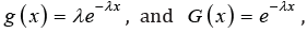 , respectively.
Additionally, the moments, the moment generating function and
several other properties of this distribution can be expressed in
terms of elementary functions [3-5].
, respectively.
Additionally, the moments, the moment generating function and
several other properties of this distribution can be expressed in
terms of elementary functions [3-5].
The cumulative distribution function 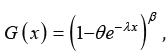 for
for 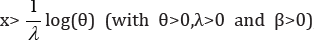 was used during the first
half of the nineteenth century by Gompertz [6] and Verhulst [7-
9] to compare known human mortality tables and to represent
population growth, respectively. Ahuja & Nash [10] also used
this model and some related models for growth curve mortality.
The Exponentiated Exponential (EE) distribution (also known
as the generalized exponential distribution) discussed in Gupta
[1], is defined as a particular case of the Gompertz-Verhulst
distribution function when θ=1, that is, the cumulative distribution
function of the EE distribution becomes The
Exponentiated Exponential distribution is also a special case of the
three-parameter exponentiated Wei bull distribution, Mudholkar &
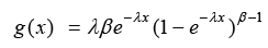
Srivastava [11]. Note that if β=1, then the EE distribution reduces
to the exponential distribution with probability density and failure
rate functions:
was used during the first
half of the nineteenth century by Gompertz [6] and Verhulst [7-
9] to compare known human mortality tables and to represent
population growth, respectively. Ahuja & Nash [10] also used
this model and some related models for growth curve mortality.
The Exponentiated Exponential (EE) distribution (also known
as the generalized exponential distribution) discussed in Gupta
[1], is defined as a particular case of the Gompertz-Verhulst
distribution function when θ=1, that is, the cumulative distribution
function of the EE distribution becomes The
Exponentiated Exponential distribution is also a special case of the
three-parameter exponentiated Wei bull distribution, Mudholkar &
Srivastava [11]. Note that if β=1, then the EE distribution reduces
to the exponential distribution with probability density and failure
rate functions:
and
Respectively, We notice that the failure rate function of the EE distribution can be increasing (for β>1) or decreasing (for β< 1). If β=1, the failure rate function becomes constant. Pointed out that the failure rate function of the EE distribution behaves like the failure rate function of the gamma distribution, and it can be used as an alternative distribution to the gamma and Wei bull distributions in many situations. Additionally, these authors derived several mathematical properties of this distribution. The EE distribution has been the subject of some research papers and has received widespread attention in the last few years. We refer the reader to Zheng [12], Gupta & Kundu [13-15], Kundu & Gupta [16], Pradhan & Kundu [17], Abdel-Hamid & Al-Hussaini [18], Aslam et al. [19] and Nadarajah [20], among many others. Nadarajah & Haghighi [21] introduced a new extension of the exponential distribution as an alternative to the gamma, Wei bull and the EE distributions. The cumulative distribution function of NH distribution is given

where λ>0 is the scale parameter and α>0 is the shape parameter. The corresponding probability density and failure rate functions are given by

and

Note that equation (2) has two parameters just like the gamma, Wei bull and the EE distributions. Note also that equation (2) has closed for survival function and hazard rate functions just like the Wei bull and the EE distributions. For α=1, (2) reduces to the exponential distribution. As we shall see later, (2) has the attractive feature of always having the zero mode and yet allowing for increasing, decreasing and constant hazard rate function [20]. Also Nadarajah & Haghighi [21] presented some motivations for introducing their new distribution.
The first motivation is based on the relationship between the probability density function in (2) and its failure rate function. The NH density function can be monotonically decreasing and yet its failure rate function can be increasing. The gamma, Wei bull and EE distributions do not allow for an increasing failure function when their respective densities are monotonically decreasing. The second motivation is related with the ability (or the inability) of the NH distribution to model data that have their mode fixed at zero. The gamma, Wei bull and EE distributions are not suitable for situations of this kind. The third motivation is based on the following mathematical relationship: if Y is a Wei bull random variable with shape parameter α and scale parameter λ, then the density in Eq. (1.2) is the same as that of the random variable Z=Y-1 truncated at zero; that is, the NH distribution can be interpreted as a truncated Wei bull distribution. For further details about this new model as well as general properties, the reader is referred to Nadarajah & Haghighi [21].
The distribution introduced by Kumaraswamy [22], also referred to as the “minimax” distribution, is not very common among statisticians and has been little explored in the literature, nor its relative inter changeability with the beta distribution has been widely appreciated. We use the term Kw distribution to denote the Kumaraswamy distribution. The Kumaraswamy (Kw) distribution is not very common among statisticians and has been little explored in the literature. Its Cumulative Distribution Function (cdf) is given by

where a>0 and b>0 are shape parameters. Equation (4) compares extremely favourably in terms of simplicity with the beta cdf which is given by the incomplete beta function ratio. The corresponding Probability Density Function (pdf) is

The Kw pdf has the same basic shape properties of the beta distribution: a>1 and b>1 (uni-modal); a<1 and b<1(uni-anti model); a>1 and b≤1(increasing); a≤1 and b>1(decreasing); a=1 and b=1(constant). It does not seem to be very familiar to statisticians and has not been investigated systematically in much detail before, nor has its relative inter changeability with the beta distribution been widely appreciated. However, in a very re- cent paper, Jones [23] explored the background and genesis of this distribution and, more importantly, made clear some similarities and differences between the beta and Kw distributions. However, the beta distribution has the following advantages over the Kw distribution: simpler formulae for moments and Moment Generating Function (mgf), a one-parameter sub-family of symmetric distributions, simpler moment estimation and more ways of generating the distribution by means of physical processes.
In this note, we combine the works of Kumaraswamy [22] to derive some mathematical properties of a new model, called the Kw-G distribution, which stems from the following general construction: if tt denotes the baseline cumulative function of a random variable, then a generalized class of distributions can be defined by

Where a>0 and b>0 are two additional shape parameters which aim to govern skewness and tail weight of the generated distribution. An attractive feature of this distribution is that the two parameters a and b can afford greater control over the weights in both tails and in its centre. The Kw-G distribution can be used quite effectively even if the data are censored. The corresponding probability density function (pdf) is

The density family (7) has many of the same properties of the class of beta-tt distributions [24], but has some advantages in terms of tractability, since it does not involve any special function such as the beta function. Equivalently, as occurs with the beta-G family of distributions, special Kw-G distributions can be generated as follows: the Kw-Wei bull [25]. General results for the Kumaraswamy distribution [26]. Kw- Ggeneralized gamma [27], Kw-G Birnbaum- Saunders [28] and Kw Gumbel [29] distributions are obtained by taking G(x) to be the cdf of the Wei bull, generalized gamma, Birnbaum-Saunders and Gumbel distributions, respectively, among several others. Hence, each new Kw-G distribution can be generated from a specified tt distribution
A physical interpretation of the Kw-G distribution given by (6) and (7) (for a and b positive integers) is as follows. Suppose a system is made of b independent components and that each component is made up of a independent subcomponents. Suppose the system fails if any of the b components fails and that each component fails if all of the subcomponents fail. Let Xj1,Xj2,...,Xja denote the life times of the subcomponents within the jth component, j=1,...,b with common (cdf) G. Let Xj denote the lifetime of the jth component, j=1,...,b and let X denote the lifetime of the entire system. Then the (cdf) of X is given by
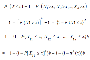
So, it follows that the Kw- G distribution given by (6) and (7) is precisely the time to failure distribution of the entire system. Now we propose the Kumaraswamy extension Exponential (denoted with the prefix KEE).
The rest of the article is organized as follows. In Section 2, we define the Kumaraswamy extension Exponential distribution, the expansion for the cumulative and density functions of the KEE distribution and some special cases. Quantile function, median, moments, moment generating functions and mean residual lifetime are discussed in Section 3. Least squares and weighted least squares estimators introduced in Section 4. Finally, maximum likelihood estimation is performed in Section 5.
Kumaraswamy Extension Exponential Distribution
In this section we studied the Kumaraswamy Extension Exponential (KEE) distribution and the sub-models of this distribution. Now using (1) and (2) in (6) we have the cdf of Kumaraswamy extension Exponential distribution

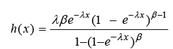
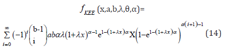
The KEE variate X following (8) is denoted by X~KEE(φ), φ=(a,b,α,λ). The corresponding probability density function (pdf) of (8) is given by

The associated survival, hazard rate and reversed hazard rate functions can be written as


Special cases of the KEE distribution
The Kumaraswamy extension Exponential (KEE) distribution is very flexible model that approaches to different distributions when its parameters are changed. In addition to some standard distribution the (KEE) distribution includes the following well known distribution as special models. If X is a random variable with cdf (8) or pdf (9) then we have the following cases
1. For b=1, then (8) reduces to A new exponential-type distribution which is introduced by Lemonte [30].
2. Applying a=b=1, we can obtain the extension Exponential distribution which is introduced by Nadarajah & Haghighi [21].
3. Kumaraswamy generalized Exponential distribution arises as a special case of KEE by taking α=1.
4. If α=1 then (8) gives Kumaraswamy exponential distribution [25].
5. For b=α=1 we get the generalized Exponential distribution which is introduced by Gupta & Kundu [1].
6. Applying a=b=α=1 we can obtain the exponential distribution [25].
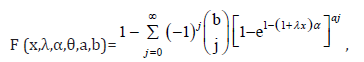
Expansion for the cumulative and density functions
In this subsection we present some representations of cdf, pdf of Kumaraswamy extension Ex-ponential distribution. The mathematical relation given below will be useful in this subsection.
By using the generalized binomial theorem if β is a positive and |z|<1, then

First, note that 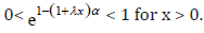 Using (13) we get
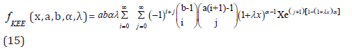
also using the power series of (13) the equation (9) becomes
Again apply (13) in the last term of (15), we obtain

Statistical Properties
In this section we studied the statistical properties of the (KEE) distribution, specifically quan- tile function, moments, incomplete moment and moment generating function.
Quantile and median
Quantile functions are used in theoretical aspects, statistical applications and Monte Carlo methods. Monte-Carlo simulations employ quantile functions to produce simulated random variables for classical and new continuous distributions. The inverse of the cdf (3) yields a very simple quantile function, say Q(u), of X is given by

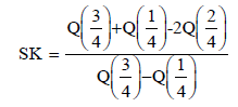
A sample from the KEE distribution may be obtained by applying its quantile function to a sample from a uniform distribution. Further, we can obtain the median, quantiles 25 and 75 by replacing 0.5, 0.25 and 0.75 in equation (17), respectively. The shortcomings of the classical kurtosis measure are well-known. There are many heavy-tailed distributions for which this measure is infinite, so it becomes uninformative precisely when it needs to be. Indeed, our motivation to use quantile-based measures stemmed from the nonexistence of classical kurtosis for many distributions. The effect of the shape parameters a and b on the skewness and kurtosis of the KEE distribution can be based on quantile measures. One of the earliest skewness measures to be suggested is the Bowley skewness, defined by
On the other hand , the Moors kurtosis (see Moors (1988)) based on cotiles is given by
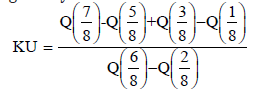
where Q(•) represents the quantile function. The measures SK and KU are less sensitive to outliers and they exist even for distributions without moments. For symmetric uni-modal distributions, positive kurtosis indicates heavy tails and peakedness relative to the normal distribution, whereas negative kurtosis indicates light tails and flatness. For the normal distribution, SK=KU=0.
The moments
Many of the interesting characteristics and features of a distribution can be studied through its moments. In this subsection, we derive the rth moments and moment generating function MX(t) of the KEE(ϕ) where ϕ=(a,b,α,λ). Let X be a random variable following the KEE distribution with parameters a,b,α and λ. Expressions for mathematical expectation, variance and the rth moment on the origin of X can be obtained using the well-known formula.
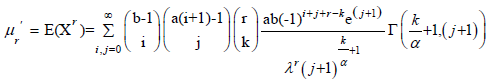
a) Lemma 1: If X has KEE(ϕ), then the rth moment of X, r=1,2,.... has the following form:
Proof
Let X be a random variable with density function (15). The rth ordinary moment of the KEE distribution is given by
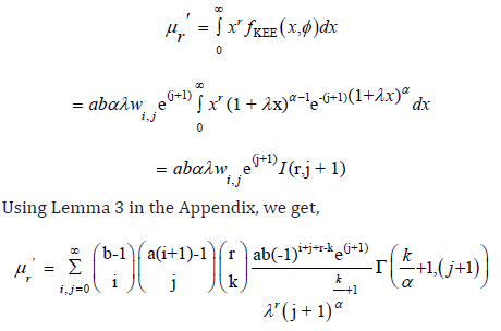
Which completes the proof
The central moments μr and cumulants Kr of the KEE distribution can be determined from expression (18) as
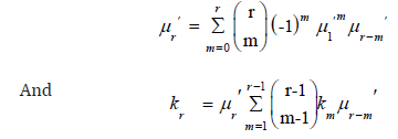
Respectively, where 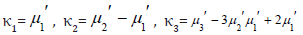
 etc. Additionally, the
skewness and kurtosis can be calculated from the third and fourth
standardized cumulants in the forms
etc. Additionally, the
skewness and kurtosis can be calculated from the third and fourth
standardized cumulants in the forms 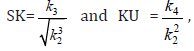 respectively.
b) Lemma 2: If X has KEE(ϕ), then the moment generating function MX(t) has the following
form
Proof
We start with the well known definition of the moment generating function given by
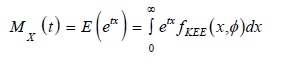
Since, converges and each term is integrable for all t
close to 0, then we can rewrite the moment generating function as
converges and each term is integrable for all t
close to 0, then we can rewrite the moment generating function as 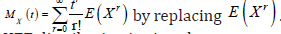 .Hence using (18) the MGF of
KEE distribution is given by
.Hence using (18) the MGF of
KEE distribution is given by
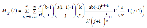
which completes the proof.
Similar, the characteristic function of the KEE distribution becomes ϕX(t) = MX(it)
where i = is the unit imaginary number.
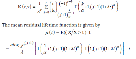
Mean residual lifetime
Given that a component survives up to time t≥0, the residual life is the period beyond t until the time of failure and defined by the conditional random variable X−t|X>t. In reliability, it is well known that the mean residual life function and ratio of two consecutive moments of residual life determine the distribution uniquely [31]. Therefore, we obtain the rth-order moment of the residual life via the general formula
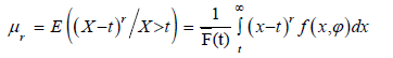
Applying the binomial expansion of (x−t)r, substituting (9) and (10) into the above formula gives

Using Lemma 4 in the Appendix, we get
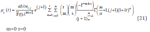
where 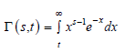
For lifetime models, it is also of interest to know what E (X r X >t ) is, Using Lemma 4
in the appendix, it is easily seen that

Where
Least Squares and Weighted Least Squares estimators
In this section we provide the regression based method estimators of the unknown parameters of the Kumaraswamy extension exponential distribution, which was originally suggested by Swain et al. [32] to estimate the parameters of beta distributions. It can be used some other cases also. Suppose Y1,....,Yn is a random sample of size n from a distribution function G(.) and suppose Y(i); i=1, 2, . . . , n denotes the ordered sample. The proposed method uses the distribution of G(Y(i)). For a sample of size n, we have
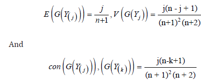
see Johnson et al. [4]. Using the expectations and the variances, two variants of the least squares methods can be used.
Method 1
(Least Squares Estimators) Obtain the estimators by minimizing

with respect to the unknown parameters. Therefore in case of KEE distribution the least squares estimators of a,b,α, and λ say aLSE, b LSE, α LSE, λLSE respectively, can be obtained by minimizing
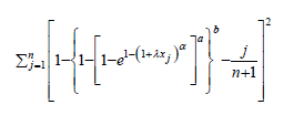
with respect to a, b, α, and λ.
Method 2
(Weighted Least Squares Estimators) The weighted least squares estimators can be obtained by minimizing

with respect to the unknown parameters, where
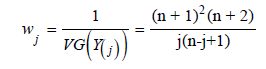
Therefore, in case of KEE distribution the weighted least squares estimators of a, b, α, and λ, say
aLSE, b LSE, α LSE, λLSE, respectively, can be obtained by minimizing
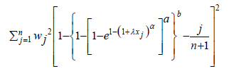
With respect to the unknown parameters only
Estimation and Inference
In this section, we derive the maximum likelihood estimates of the unknown parameters ϕ=(a,b,α,λ) of KEE distribution based on a complete sample. Let us assume that we have a simple random sample X1, X2,...,Xn from KEE(a,b,α,λ). The likelihood function of this sample is

Substituting from (9) into (26), we get

The log-likelihood function for the vector of parameters ϕ=(a,b,α,λ) can be written as

The log-likelihood can be maximized either directly or by solving the nonlinear likelihood equa- tions obtained by differentiating (28). The components of the score vector W(ϕ) are given by

We can find the estimates of the unknown parameters by maximum likelihood method by setting these above non-linear equations (29)-(32) to zero and solve them simultaneously.
Simulation Study
In order to study the behavior of the MLEs, this section presents the results of a Monte Carlo experiment on finite samples. For this study we consider seven different set of parameters for n=50,80,100,150,200,400 and 800 generated according to a TGL distribution. Note that, generated for each value of the KEE distribution, we had to solve a nonlinear equation by the Newton Raphson method. All results were obtained from 1,000 Monte Carlo replications and fixed λ=α=0.5.
Table 1:Estimated parameter values and errors for different values of the a and b parameters and different sample sizes.

Table 2:Coverage Probability and MSE of a and b parameters and different sample sizes.

The results are summarized in two tables. Table 1 shows the generated and estimated parameter values and their respectively errors over the 1, 000 MLEs, which are observed to decay as the sample size increases. Table 2 shows the coverage probability of a 95% two sided confidence intervals for the model parameters and the mean square errors, which are observed to decay as the sample size increases as the estimated errors.
Conclusion
In this paper we propose a new distribution based on the Kumaraswamy distribution Jones [23], the Kumaraswamy Extension Exponential Distribution (KEE). The proposed distribution is very flexible model that approaches to different distributions when its parameters are changed such as: a new exponential-type distribution which is introduced by Lemonte [30] the extension Exponential distribution which is introduced by Lemonte [30], Kumaraswamy generalized Exponential and Kumaraswamy exponential distribution [25] generalized Exponential introduced by Gupta & Kundu [1] and exponential distribution [25]. Some mathematical properties along with order statistics and estimation issues are addressed and a simulation study was made.
References
- Gupta RD, Kundu D (1999) Generalized exponential distribution. Austral & New Zealand Journal of Statistics 41: 173-188.
- Nadarajah S, Kotz S (2006) The exponentiated type distributions. Acta Applicandae Mathematicae 92(2): 97-111.
- Marshall AW, Olkin I (2007) Life Distributions: structure of nonparametric, semipara metric and parametric families. Springer, ISBN: 978-0-387- 68477-2.
- Johnson N, Kotz S, Balakrishnan N (1994) Continuous Univariate Distributions, volume 1, Wiley, p. 784.
- Balakrishnan N, Basu A (1995) The exponential distribution. Theory Methods and Application, Gordon and Breach Science Publishers, USA.
- Gompertz B (1825) On the nature of the function expressive of the law of human mortality, and on a new mode of determining the value of life contingencies. Philosophical Transactions of the Royal Society of London 115(1825): 513-585.
- Verhulst PF (1838) Notice sur la loi que la population suit dans son accroissement. Curr Math Phys 10(1838): 113-121.
- Verhulst PF (1845) Nouvelles memoires de l’academie royale des sciencs et belles-lettres de bruxelles. 18: (38).
- Verhulst PF (1847) Deuxieme memoire sur la loi d’accroissement de la population, Memoires de l’Academie Royale des Sciences, des Lettres et des Beaux-Arts de Belgique. EuDML 20: 1-32.
- Ahuja JC, Nash SW (1967) The generalized gompertz verhulst family of distributions. Sankhya The Indian Journal of Statistics, Series A 29(2): 141-156.
- Mudholkar G, Srivastava DK (1993) Exponentiated Weibull family for analyzing bathtub failure-rate data. IEEE Transactions on Reliability 42(2): 299-302.
- Zheng G (2002) Fisher information matrix in type-II censored data from exponentiated exponential family. Biometrical Journal 44(3): 353-357.
- Gupta RD, Kundu D (2001) Exponentiated exponential family: an alternative to gamma and Weibull distributions. Biometrical Journal 43(1): 117-130.
- Gupta RD, Kundu D (2003) Discriminating between the Weibull and the GE distributions. Computational Statistics and Data Analysis 43(2): 179- 196.
- Gupta RD, Kundu D (2007) Generalized exponential distribution: existing methods and recent developments. Journal of Statistical Planning and Inference 137(11): 3537-3547.
- Kundu D, Gupta R D (2008) Generalized exponential distribution: Bayesian estimations. Computational Statistics and Data Analysis 52(4): 1873-1883.
- Pradhan B, Kundu D (2009) On progressively censored generalized exponential distribution. Test 18: 497-515.
- Abdel Hamid AH, Al Hussaini EK (2009) Estimation in step-stress accelerated life tests for the exponentiated exponential distribution with type-I censoring. Computational Statistics and Data Analysis 53(4): 1328-1338.
- Aslam M, Kundu D, Ahmad M (2010) Time truncated acceptance sampling plans for generalized exponential distribution. Journal of Applied Statistics 37: 555-566.
- Nadarajah S (2011) The exponentiated exponential distribution: a survey. AStA Advances in Statistical Analysis 95: 219-251.
- Nadarajah S, Haghighi F (2011) An extension of the exponential distribution. Statistics 45: 543-558.
- Kumaraswamy P (1980) A generalized probability density function for double bounded random processes. Journal of Hydrology 46(1-2): 79-88.
- Jones MC (2009) A beta- type distribution with some tractability advantages. Statistical Methodology 6: 70-81.
- Eugene N, Lee C, Famoye F (2002) Beta-normal distribution and its applications. Communications in Statistics Theory and Methods 31: 497-512.
- Cordeiro GM, Ortega EMM, Nadarajah S (2010) Kumaraswamy Weibull distribution with application to failure data. Journal of the Franklin Institute 347(8): 1399-1429.
- Nadarajah S, Cordeiro GM, Ortega EMM (2012) General results for the Kumaraswamy-G distribution. Journal of Statistical Computation and Simulation 82(7): 951-979.
- Pascoa ARM, Ortega EMM, Cordeiro GM (2011) The kumaraswamy generalized gamma distribution with application in survival analysis. Statistical Methodology 8(5): 411-433.
- Saulo H, Bourguignon M (2012) The Kumaraswamy birnbaum-saunders distribution. Statistical Methods & Applications 21(2): 139-168.
- Cordeiro GM, Nadarajah S, Ortega EMM (2012) The Kumaraswamy gumbel distribution. Statistical Methods and Applications 21: 139-168.
- Lemonte AJ (2013) A new exponential-type distribution with constant, decreasing, increasing, upside-down bathtub and bathtub-shaped failure rate function. Computational Statistics and Data Analysis 62: 149-170.
- Gupta RC, Gupta RD (1988) On the distribution of order statistics for a random sample size. Statist Neelandica 38: 13-19.
- Swain JJ, Venkatraman S, Wilson JR (1988) Least-squares estimation of distribution functions in Johnson’s translation system. Journal of Statistical Computation and Simulation 29: 271-296.
© 2018 Francisco Louzada. This is an open access article distributed under the terms of the Creative Commons Attribution License , which permits unrestricted use, distribution, and build upon your work non-commercially.
Editor In Chief


.jpg)


Signup for Newsletter

Quick Links
 Editorial Board Registrations
 Submit your Article
 Refer a Friend
 Advertise With Us
Our Recent Edition

.jpg)


Top Editors


.jpg)


.bmp)
.jpg)
.png)
.jpg)


.jpg)


.png)

.png)


.png)


Financial Support

Sponsors

Latest e-Books

Latest Video

 a Creative Commons Attribution 4.0 International License. Based on a work at www.crimsonpublishers.com.
Best viewed in
a Creative Commons Attribution 4.0 International License. Based on a work at www.crimsonpublishers.com.
Best viewed in