Speed of Road Traffic for Optimal Climate Protection

When designing road traffic, one prescribes the traffic speed according to the external conditions. These can be diverse, for example roadway properties (geometry, surface structure), roadway environment, weather conditions, safety, environmental protection, etc. For traffic safety and noise reduction, the traffic speed is usually limited, whereby the traffic is calmed (smoothed). This measure has proven itself many times in practice. Motivated by the fact that fuel consumption in road traffic depends on the driving speed, namely the flow rate of fuel leaving the fuel tank increases with increasing driving speed, it has been concluded that a reduction in traffic speed could also reduce fuel consumption. This conclusion remains an immovable truth, not only among decision-makers, but also among transport designers with regard to climate and environmental protection. As far as the author is aware, no one has questioned this conclusion or considered it to be untenable. Numerous measures known under the collective term speed limit, for example Tempo30, are based on this conclusion. In the following it will be shown that by limiting the traffic speed, not all conditions can be met simultaneously, which one places on the road traffic. For example, the speed limit significantly increases traffic safety, but can increase fuel consumption thus reducing the climate protection in comparison to a higher speed case.

Fuel consumption and traffic speeds

From recent studies we can conclude that at a certain traffic speed w_opt there should be a minimum of fuel consumption Q_min. From the results reported by Mitrovic [1], we can establish the diagram depicted in Figure 1. The diagram shows the fuel consumption (flow rate of fuel leaving the fuel tank) V [l / h] as function of traffic speed w; V₀ at w → 0 corresponds to the idling fuel consumption of the engine. The quantity τ shown in the diagram denotes the time required to travel the section of the length L at the speed w.

We limit the considerations to the case of a constant traffic speed w on the section L. In this case the volumetric floe rate of fuel V [l / h] is also constant and the fuel consumption on the distance L follows from

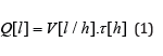
The boundary condition to be satisfied by this equation are:
Idling of engine

Large traffic speed

For very low traffic speed w → 0 ( ≈ idling of engine) both the time τ and the fuel consumption Q[l] are very large: τ → ∞,Q[l]→ ∞ . A numerical value of fuel consumption at large but finite traffic speed, Eq. (3), the fuel consumption is also large and finite Q[l]→ finite . In this case the fuel consumption, taken as the product of a large fuel flow rate V[l/h] and a small driving time τ , will give a finite value of Q[l] which must be determined from experiments. However, a precise determination of Q[l] at large w is not necessary if we are to show that Q[l] in Eq. (1) has a minimum, as demonstrated in [1] and illustrated in Figure 2 below.

The diagram applies to the travel on a section L of the route that leads from one place (A) to the other place (B). The driving on this section takes place at constant speed w without disturbances, the speed w is varied as a parameter in the model [2,3].

Corresponding to the minimum of the Q[l] -curve in Figure 1 the formation and emission of combustion gases to the environment and thus its pollution is minimal. Every trip at a speed w different of w_opt , w ≠ w_opt , results in a higher fuel consumption, Q > Q_min. From the point of view of fuel consumption and climate protection, it is important to determine the fuel requirement Q at the actual speedw and minimize the difference ΔQ = Q − Q_min by suitable measures.

Figure 1:Illustration of variables relevant for climate protection in road traffic.

It is advisable to carry out the analysis for 2 cases:
i. Case a: The actual driving speed w is below the speed w_opt,W < w_opt
ii. Case b: The actual driving speed w is above the speed w_opt, w > w_opt .

TheQ[l] - curve in Figure 1 immediately shows the way how to reduce the fuel consumption impact of traffic on the climate. In the speed region w < w_opt , the traffic speed must be increased, whereas for w > w_opt a speed reduction is required. Next, we quantify the additional fuel consumption when driving at speeds different from wopt confining ourselves to the region of w < w_opt . This should illustrate what actually happens when the speed is reduced intentionally like in a tempo limit zones or in traffic congestion zone formed occasionally by traffic disturbances.

Basic dependencies

Figure 2, taken from [1] and modified, illustrates the basic dependencies with 2 different gear shifts for the car VW Golf 1.4 TSI of 90 kW engine power. The fuel consumption is shown as a function of the traffic speed. The cars form a homogeneous stream on a road section of the length L = 10km (comparable to a train composition). The distance between the cars that includes the safety distance plus the car length depends on the driving speed w, l = k ⋅ w , k being a constant that is varied as a parameter. At given k, the distance l increases along the w axis at the speed w. The fuel consumption QN represents the amount of fuel which all vehicles (index N) that are currently on the section L consume when they cover this section and move at the speed w. The pollution of the environment by traffic emissions adjusts itself according to the fuel consumption. The QN -curve contains only quantities which are accessible by experiments. These conditions define an ideal traffic model.

Figure 2:Fuel consumption as a function of the traffic speed with 2 gear positions.

Traffic speed at fuel consumption minimum

When driving in 3^rd gear (Figure 2 left), fuel consumption decreases with increasing speed w and at w ≈ 80km / h it reaches values that only depend on k. The safety distance according to an empirical rule corresponds to the value k = 0.5 and the following considerations will refer to this value of k. At a smaller value k, the safety distance l between the cars is smaller and the number of cars on the section L, and thus also the fuel consumption QN , is larger. When driving in 5^th gear (Figure 2 right), the fuel consumption passes through a pronounced minimum at w = w_opt ≈ 100km / h . Viewed from the standpoint of climate protection and energy requirements, the traffic should neither exceed nor significantly fall below the optimum speed w_opt.

Minimum of fuel consumption

The minimum fuel consumption Q_min for driving in 3^rd gear at k = 0.5 is Q _min = 150 litres . The same quantity for the 5^th gear and k = 0.5 amounts to Q _min = 110 litres , that is, more than 26% less than that in 3^rd gear, (Figure 2). Driving in 3^rd gear should therefore be avoided.

Fuel consumption at Tempo30

For driving in 3^rd gear on the same route L not at the optimal speed ( w = 100km / h ), but at w = 30km / h (Tempo30), the fuel consumption increases from 150 litres to around 290 litres, that is, by the factor of

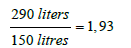
or by 93%. From a climate protection point of view, this increase is surprising high. In other words, assuming the quality of the engine combustion of the fuel to be independent of the driving speed, the impact of exhaust gases on environment when driving in 3^rd gear at Tempo30 ( w = 30km / h ), compared to the impact when driving in the same gear at the optimal speed between 80 km / h to 100 km / h , increases by a factor of 1.93.

The situation becomes even more dramatic if the diving at the optimum speed is not in 3^rd gear but in 5th gear at a speed of 100 km / h at the fuel minimum of around 110 litres, (Figure 2) on the right. In this case, the fuel consumption increases by the factor of

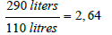
when driving at the speed w = 30 km / h in 3^rd gear, or by 164%.

These results lead to the conclusion that the speed reduction with regard to climate protection in case a), i.e. at traffic speeds below the speed of the fuel minimum, are counterproductive. A reduction in speed in this area leads to increased fuel consumption and to a greater environmental pollution. On the other hand, in case b), at speeds above the optimal speed (Figure 2 right), the speed limit is generally recommended. Here, however, the increase in fuel consumption with increasing traffic speed is significantly less than in the case of speed zones at low traffic speeds, Case a).

Electric cars

The fuel consumption according to Figure 1 is a general characteristic of road traffic. A minimum of the fuel requirement is to be expected with all car types, even if the speed at which the minimum occurs will be car-specific. The form of the energy demand in (Figure 1) is expected also for electric cars, because the external resistances dominate the fuel (energy) requirement. These resistances are independent of the kind of energy employed to drive the cars. As long as this energy is obtained from natural energy sources, such as solar radiation, hydro and aero energy, traffic will not directly pollute the climate with combustion products. In this case, the energy taken up by traffic from natural sources is converted into another form required by traffic, dissipated and given off as heat with a lower driving temperature difference to the environment.

Our results can be summarized as follows:
a. With regard to fuel consumption and environmental protection, speed zones with low traffic speeds (e.g. Tempo30) cannot be recommended as effective measures.
b. When planning speed limited zones, their opposing effects must be carefully weighed against each other. These are on the one hand the positive effects of traffic safety and on the other hand the negative effects of the increased pollution of the living space by combustion products.
c. These considerations explain the enormous environmental pollution in metropolitan areas through zones of low speed, which inevitably lead to greater traffic density and thus to an overloading of the air with exhaust gases. It is irrelevant whether such zones are caused intentionally (traffic planning) or by the traffic congestion.
d. The additional fuel requirement due to speed reduction should also be examined economically. This also applies to electric cars, which do not immediately emit any exhaust gases, but require more energy through speed zones.

Letters in brackets denote units
L - travel distance
l - car distance (includes safety distance & car length)
Q - fuel consumed on L
t - time
V - flow rate, consumed fuel
V₀ - idling fuel consumption
w - traffic speed
τ - travel time on L

1. Mitrovic J (2020) Optimal speed of road vehicles with regard to fuel consumption. Emission Control 25: 20-25.
2. Barth M, Boriboonsomsin K (2009) Traffic congestion and greenhouse gases. Magazine 1 35: 2-9.
3. Barth M, Boriboonsomsin K (2008) Real-World CO₂ Impacts of Traffic Congestion. Transportation Research Record. Journal of the Transportation Research Board, Transportation Research Board, National Academy of Science, pp. 1-23.