
- About Us
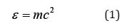
- Information
-

The Author ensures that the research has been conducted responsibly and ethically with adherence to all relevant regulations. read more..
- For Authors
- For Reviewer
- Manuscript Guidelines
- Membership
- Publication Ethics
-
- Journals
- Reprints
- e-Books
- Videos
- Policies
- Contact Us
 COVID-19
- Submissions


Full Text
Novel Research in Sciences
Case Report: Abdominal Aortic Aneurysms
Janusz Wolny* and Radoslaw Strzalka
Faculty of Physics and Applied Computer Science, AGH University of Science and Technology, Krakow, Poland
*Corresponding author: Janusz Wolny, Faculty of Physics and Applied Computer Science, AGH University of Science and Technology, Krakow, Poland
Submission: February 26, 2021;Published: March 03, 2021
.jpg)
Volume6 Issue1March, 2021
Abstract
The paper presents a way to generalize a relativistic equation of dynamics to describe the movement of a material particle in a force field with moving sources. In the static force field version, the equation is identical to the standard equation of dynamics in special relativity. The same formula can also be derived from the equation of motion for variable-mass systems with the additional assumption of the energy-mass equivalence, instead of assuming the constancy of the speed of light. A new approach to the dynamics of relativistic objects makes it possible to describe the magnetic interaction associated with the electric current of moving charges.
Keywords: Magnetic force; Relativistic dynamics
Introduction
In special relativity, the kinematics of moving objects is ruled by the Lorentz transformation of time and space components [1]. In the modern approach, to describe objects at relativistic speeds, a 4-dimensional Minkovsky spacetime, as well as an energy-momentum 4-vector are used [2]. The dynamics (force) are usually described by a relativistic generalization of the Newtonian Second Law with a proper time τ used instead of ‘regular’ time t. The correct description of the components of force and acceleration is obtained using the relativistic transformation. In our previous work, we showed that using Lorentz transformation is not necessary to correctly describe the dynamics of objects in motion, and the results known from special relativity can be obtained when starting from a classical mechanics [3]. The same applies to the problem of a particle undergoing an influence of external moving force field’s sources. Special relativity properly explains electric and magnetic phenomena and predicts the definition of forces (Lorentz force law) via electromagnetic field tensor. As we know, the success of the theory of special relativity comes also from the Lorentzian invariance of Maxwell equations of electromagnetism. In this paper we want to show, that, again, starting from completely classical mechanics, the very same (correct and compatible with special relativity) results can be obtained for describing a motion of particles under external fields.
A Different Derivation of the Relativistic Equation of Motion
In the present work, we use a new approach to describe the dynamics of objects in motion, both classical and relativistic, based on the equation of motion for objects with variable mass [4]. Derivation of the relativistic equation of dynamics was based on two assumptions. The first is the equivalence of mass (m) and energy (ε ) expressed for a vacuum with the famous Einstein’s equation:
In this equation, the value of C2 is a constant parameter, characteristic for vacuum. The mass of the object changes as the energy of the moving (ε0) particle changes. Energy (ε ) is energy in motion and contains the rest energy (ε0) and the kinetic energy of a material point with a constant rest mass m0 , the variable mass of which in motion is m. We assume that the energy of the particle changes only through the power of the force acting on the object supplied to the system. Force power is the scalar product of the force vector and the velocity vector of the body, calculated in relation to the stationary source of force. Other energy change channels (including rotational energy, or the internal energy of the system in general) are not considered.
In turn, the dynamic equation of motion for an object with constant rest mass is expressed by the formula (see the discussion of the general equation of motion for variable mass systems in [4]):
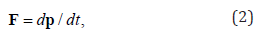
meaning that a force F applied to an object causes a change in time of a momentum (p = mv)
As a result of the force acting on a body, its energy changes according to the relation (which is known as energy-work theorem):
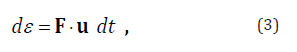
where u is the velocity vector of the body relative to the motion of the force’s source, and the product of force and relative velocity (F⋅u) expresses the power supplied to the system from the source of the force.
Combining the above three equations (1)-(3) we obtain a relativistic equation of motion:
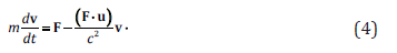
The result in (4) was already showed in [4]. If in the chosen laboratory system (LAB) the particle’s velocity is v, and the velocity of the force’s source is v0 , then u = v − v0 and the equation of dynamics is expressed by the formula:
and this is the dynamic equation of motion for the object with a constant rest mass moving in the force field F , whose source moves at the speed v0.
Equation (5) can be generalized to motion in a field of many forces:
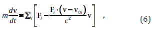
where v0i are the velocity vectors of sources of forces Fi .
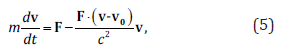
The equation of dynamics (5) can also be simplified to the case of a resting source of force and then it is reduced to the equation:
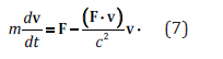
Equation (7) is identical to the equation derived within the special theory of relativity. It should be noted, however, that this time we do not use postulates of special relativity, namely the speed of light postulate or description in Minkowski 4-dimensional spacetime. Using equation (7) it can be shown [3] that c is the critical velocity for the motion of a particle, for which the particle’s energy, and thus its mass in motion, reaches an infinite value. Therefore, speed c delimits the speed of the particle into two areas: sub- and superluminal. These areas are well separated and do not mix with each other. In both areas, the energy-momentum invariants hold, as is the case in special relativity [3].
The essential difference comparing to special relativity appears for moving force fields’ sources. To this end, we will analyze a simple model example. For simplicity, we assume a one-dimensional motion for which the velocity is parallel to the acting force and u is parallel to v. In this case equation (4) can be simplified to the form:
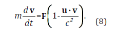
We can determine the critical velocity values by comparing the derivative dv/dt to 0, which leads to the equation:
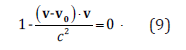
The solution to the quadratic equation (9) is:
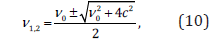
which is also depicted in Figure 1. It should be noted that only for v0 =0 we have a symmetrical solution,v1 =-v2 =C . This is also the case described by special relativity. For non-zero values of v0 , the symmetry is broken. For small values of the ratio v0/c formula(10) can be replaced by:
Figure 1:Asymptotic behavior of equation (8) leads to a dependence of the critical velocity of an object on the velocity of the field’s source,v(v0). The critical speed is c only, if V0=0.

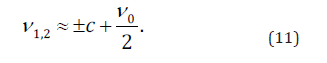
The symmetry breaking can be seen even better after transforming the equation (8) to a form:
where both mass and force were expressed by energy, m=e/c2 and F⋅u dt=dε. Finally, by integrating equation (12) we get:
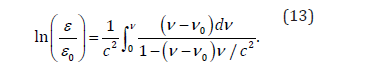
The integral in (13) can be obtained analytically, and it gives:
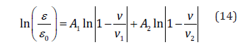
With 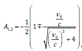 ,and
,and 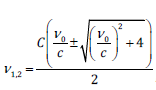 ,according
to (10). It can be shown that, indeed, symmetry in relation e(v)
is broken due to asymmetry in v1 and v2 , as well as in amplitudes A1
and A2(Figure 2). It can be seen that the average amplitude(A1+A2)/2
is constant and equal to 0.5, but the discrepancy in amplitudes is
growing with v0 . Also, positions of the asymptotes (v1 and v2) move
away from each other as v0 grows.
,according
to (10). It can be shown that, indeed, symmetry in relation e(v)
is broken due to asymmetry in v1 and v2 , as well as in amplitudes A1
and A2(Figure 2). It can be seen that the average amplitude(A1+A2)/2
is constant and equal to 0.5, but the discrepancy in amplitudes is
growing with v0 . Also, positions of the asymptotes (v1 and v2) move
away from each other as v0 grows.
Figure 2:The solution of equation (13) given by equation (14). An increasing symmetry breaking in critical speed is seen for growing speeds of a source,v0, according to (10). The energy barrier is also asymmetric for motion along v0 or in the opposite direction.

For v0 =0 the solution of equation (13) is the well-known in special relativity definition of the relativistic energy:
where  is the relativistic Lorentz factor, and e0 is the
rest energy (stored in a body at speed v0). The energy dependence
on speed (15) is fully symmetrical. The amplitudes in equation
(14) are both equal to 0.5. The particle can move only with speeds
within limits (-c,c) and it is a result completely consistent with
special relativity.
is the relativistic Lorentz factor, and e0 is the
rest energy (stored in a body at speed v0). The energy dependence
on speed (15) is fully symmetrical. The amplitudes in equation
(14) are both equal to 0.5. The particle can move only with speeds
within limits (-c,c) and it is a result completely consistent with
special relativity.
The solutions of equation (13) in the form of the equation (14)
for a static source and a moving source are shown in Figure 2. This
relation shows critical behavior but for slightly changed critical
speed values, which depend on the speed of the moving source ( ) 0 v .
For the non-relativistic range of speeds 0 v , the change in the critical
speed value is insignificant and very difficult to measure. It is also
worth to note that the particle’s energy minimum in the presence
of the moving source field  is lower than e0 (understood as
the particle’s energy at the speed v=0, relative to the LAB system).
By e we measure the energy delivered by a moving force field,
thus, the lowest energy of the particle with respect to the force field
must be achieved at v=v0, which is confirmed by Figure 2.
is lower than e0 (understood as
the particle’s energy at the speed v=0, relative to the LAB system).
By e we measure the energy delivered by a moving force field,
thus, the lowest energy of the particle with respect to the force field
must be achieved at v=v0, which is confirmed by Figure 2.
In the following, we will use a vector identity known in Euclidean 3D space (vector triple product):
Applying (16) to the dynamic equation of motion (6) gives:
After introducing a new set of Lorentz factors:
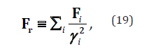
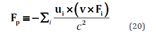
we define 2 components of the net force, denoted Fr , and Fp :
For stationary sources of force fields, the parameters gi become equal to g , and all relative velocities ui become equal to the particle velocity v . Thus, for a static source of force, equation (17) reduces to the commonly known relativistic equation of motion (7).
Force acting on a charge in the presence of moving fields
In many textbooks, the electric field and magnetic field are considered separate physical instances, although clearly distinguished experimentally. Theoretically, the electromagnetic field is usually described by a Lorentz force law, which not always is justified in textbooks, e.g. [5,6]. The common derivations of the Lorentz force usually involve the assumptions coming from the special relativity. The starting point can be either the Coulomb force undergoing the relativistic (Lorentz) transformations [7], or 4-vector generalization of the electrostatic and magnetic field (electromagnetic field tensor) [1,8,9]. We will now use a different approach. One of the more important applications of the relativistic equation of dynamics (17) is deriving the magnetic force acting on a moving charge. We know from Ampere’s empirical law that a vortex magnetic field B arises around a rectilinear conductor with a current I . This field can be derived from equation (17), what is discussed in the following parts of the paper.
Example: Magnetic field around a rectilinear conductor with current
The second component of the force,Fp, is responsible for the appearance of the magnetic field accompanying the moving charges. A point charge q moves at velocity v along a rectilinear conductor in which an electric current of intensity I flows. In a conductor, the current is caused by the movement of free electrons, moving at an average speed of v0−=ve, directed against the direction of the current flow, due to the negative value of the charge of the carriers(q− = −e where e is the elementary charge). To simplify the calculations, we assume that all current carriers move at the same and constant speed equal to ve. In the LAB system, we deal with both moving force field sources (the movement of free electrons responsible for the flow of electric current I ) and the movement of a point charge q , with the velocity v with respect to a stationary conductor.
Within the model under consideration, our ideal conductor consists of stationary cations and freely moving electrons. Linear charge densities, λ+ and λ− (the amount of charge per unit length), satisfy the relation: λ++λ− =0 (in the LAB system the conductor is uncharged). Each of the charge distribution creates an associated electric field calculated from Gauss’s law: E+ = λ+/2πε0 r, E− = λ−/2πε0 r , where r is the distance from the point to the conductor. The resulting electric field E = E+ + E− =0. All the fields considered above are perpendicular to the linear conductor.
So, we have a sum of two interactions, one with a field due to positive charges and the other with a field due to negative charges (electrons). In the model case under consideration, we have for cations u1 =v, and for electrons u2 = v− ve. The component Fp of the total force, given by (17), is thus expressed by the formula:
For the considered case ve⋅E/+− =0 and v⋅E/+− =0, so we can convert the velocity vectors into a vector triple product, which gives:
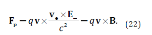
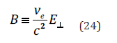
The magnetic induction vector B, defined by equation (22), is directly related to the movement of the current carriers, and thus to the intensity of the flowing current I . For the considered model, B is:
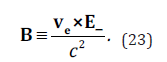
The result is fully compatible with the prediction of relativitybased formulation of electromagnetism (via electromagnetic field tensor). The value of the length of the field induction vector B depends only on the electric field component perpendicular to the electron velocity, ve , and is expressed by the formula:
The force Fp expressed by the formula (22) is called the Lorentz force for a point charge moving in a magnetic field with induction B. In turn, the intensity of the current for free electrons moving in a conductive rectilinear wire with speed v0− = ve is: I = λ− ve. Thus,the value of the magnetic field induction vector can be written as:
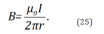
The above formula expresses the value of the magnetic field induction at a distance r from an infinitely long conductor with an electric current of intensity I , and is associated with the Ampere law. Note that the magnetic field, B, is a rotational (divergencefree) vector field complying with Gauss’s and Ampere’s laws for a magnetic field. It is not a “new” field, but an appropriately transformed electric field. The Eand B fields are related to each other. We often use the historical name electromagnetic field to describe these fields, which is somewhat misleading from the point of view of the above conclusions. The magnetic field B is closely related to the second force component,Fp , in the relativistic equation of dynamics for moving force sources (6). Both the first force component,Fr , and the second force component, Fp , depend on one and the same electric field E. The only existing field is therefore the electric field, which through the force component Fp simulates the existence of another field - the field of the magnetic induction vector. No wonder then that the E and B fields are closely related. There is no limit to the E-field, it can be both divergent and rotational, it can be anything. In turn, the magnetic field, B, is defined by equation (23) and is by definition a divergent-free (rotational) field.
Summary
The relativistic equation of dynamics (3) can be obtained both within the theory of special relativity and an alternative method based on the dynamic equation of motion for systems with variable mass. The latter method does not require the use of fourdimensional space-time and the assumption that the speed of light is constant. On the other hand, it uses the relationship between energy and mass of an object in motion, which is well-documented experimentally and also theoretically confirmed within special relativity, expressed for a vacuum using the Einstein’s formula (1). When using simple vector identities, the dynamic equation of motion can be written by the formula (6). There are two force components in this equation, the values of which depend both on the force itself and on the respective relativistic weights. The first component is the real force scaled using the Lorentz factors. The solutions of the dynamic equation of motion limited to the first component, in the non-relativistic speed range, practically do not differ from the classical results. The second component, on the other hand, has a typically relativistic basis and disappears in the classical range, and it dominates as you approach the speed of light. The force field of the second component is rotational and is substantially different from the first component.
The dynamic equation of motion obtained in this way can be generalized to cases where the sources of forces move, as is the case for a conductor in which an electric current flow. The second component of the force (the so-called precession force) allows for the definition of a new interaction - the magnetic interaction. Within the three-dimensional physical space, the formulas for the magnetic field induction vector and the magnetic force, i.e., the Lorentz force, were derived.
From our derivation a magnetic field (magnetic force) can be understood as a result of only the electric field, which is created by electric charges. In many works and lectures, an interpretation of the actual force (being an electric or a magnetic or the mix of the two) is related to the frame of reference, involving relativistic effects, like Lorentz-Fitzgerald contraction of length [10-12]. The interpretative look on the electromagnetism is, in our opinion, not a good approach. Instead, we claim the electric field being an original one, whereas magnetism is its derivative. This is, of course, not a new idea [6]. In our derivation, we however completely resign of special relativity (except for the mass-energy equivalence) and use only classical mechanics to derive forces acting on objects in external fields.
In literature a discussion can be met on what physical significance should be put on (experimentally accessible) magnetic and electric fields, and what on the (more abstract and mathematical) 4-vector potential [8,13,14]. We present a force-based approach resigning of 4-vector potentials and assuming no special relativity-related phenomena, like relativistic proper time or length contraction. The only assumptions we make are that the energy (equivalent to the object’s mass in motion, equation (1)) is delivered to the system by an external force, and the dynamics can be described by simple Newton’s Second Law (equation (2)). The system is open; energy and momentum (and also charge) are not conserved. The Lorentz force is, however, applicable to the problem of a charge moving in the presence of external moving field sources [15].
References
- Landau LD, Lifszyc EM (2010) The classical theory of fields. Oxford, United Kingdom, p. 24.
- Rindler W (2006) Essential relativity: Special, general, and cosmological. (2nd edn), OUP Oxford, United Kingdom.
- Wolny J, Strzałka R (2020) Description of the motion of objects with sub-and superluminal speeds. Am J Phys Appl 8(2): 25-28.
- Wolny J, Strzałka R (2019) Momentum in the dynamics of variable-mass systems: Classical and relativistic case. Acta Phys Pol A 135(3): 475-479.
- Jackson JD (1990) Classical electrodynamics. (3rd edn), Wiley, New York, USA.
- Feynman RP, Leighton RB, Sands M (2020) The feynman lectures on physics.
- Lorrain P, Corson DR, Lorrain F (1988) Electromagnetic fields and waves. In: Freeman WH, (3rd edn), Section 16.5, Newyork, USA, p. 291.
- Field JH (2006) Derivation of the Iorentz force law, the magnetic field concept and the Faraday-Lenz and magnetic Gauss laws using an invariant formulation of the Iorentz transformation. Phys Scr 73(6): 639-647.
- Field JH (2001) Space-time exchange invariance: Special relativity as a symmetry principle. Am J Phys 69: 569.
- Martin R (2020) Introductory physics-building models to describe our world.
- Tong D (2015) Lectures on electromagnetism. Univeristy of Cambridge, UK.
- Feynman RP, Leighton RB, Sands M (2019) The Feynman lectures on physics. pp. 13-6.
- Rohrlich F (1990) Classical charged particles. Addison-Wesley, Reading, MA, USA, p. 65.
- Ganley WP (1963) Forces and fields in special relativity. Am J Phys 31: 510.
- Mansuripur M (2012) Trouble with the Iorentz law of force: Incompatibility with special relativity and momentum conservation. Phys Rev Lett 108: 193901.
© 2021 Janusz Wolny. This is an open access article distributed under the terms of the Creative Commons Attribution License , which permits unrestricted use, distribution, and build upon your work non-commercially.
Editor In Chief


.jpg)


Signup for Newsletter

Quick Links
 Editorial Board Registrations
 Submit your Article
 Refer a Friend
 Advertise With Us
Our Recent Edition

.jpg)


Top Editors


.jpg)


.bmp)
.jpg)
.png)
.jpg)


.jpg)


.png)

.png)


.png)


Financial Support

Sponsors

Latest e-Books

Latest Video

 a Creative Commons Attribution 4.0 International License. Based on a work at www.crimsonpublishers.com.
Best viewed in
a Creative Commons Attribution 4.0 International License. Based on a work at www.crimsonpublishers.com.
Best viewed in