
- About Us
- Information
-

The Author ensures that the research has been conducted responsibly and ethically with adherence to all relevant regulations. read more..
- For Authors
- For Reviewer
- Manuscript Guidelines
- Membership
- Publication Ethics
-
- Journals
- Reprints
- e-Books
- Videos
- Policies
- Contact Us
 COVID-19
- Submissions


Full Text
Modern Concepts & Developments in Agronomy
Climate and Water Quality Policy Design for Agriculture with Environmental Co-Benefits
Asta Ervola1, Jussi Lankoski2 and Markku Ollikainen3*
1 Department of Economics and Management, University of Helsinki, Finland
2 Finnish Forest Service, Finland
3 Trade and Agriculture Directorate, France
*Corresponding author: Gojiya DK, Junagadh Agriculture University, Junagadh, Gujarath, India
Submission: April 19, 2018;Published: July 06, 2018

ISSN 2637-7659Volume3 Issue1
Abstract
Many Agro-environmental practices, such as reduced fertilizer use or establishment of green set-asides, which are incentivised by policy instruments, may have simultaneous positive effects on multiple environmental goods. These environmental co-benefits increase the social desirability of a given policy instrument. In this paper we focus on water quality and GHG emissions and examine how climate and water quality policy instruments affect both their primary target emission and co-benefit emissions. We trace out especially the relative role of land use versus input use in emissions reduction. To facilitate this comparison, we define the socially optimal policy instruments when environmental co-benefits are either accounted for or omitted.
Simulations for the Finnish agriculture show that if only water quality damage is internalised then the divergence from social optimum where both damages are internalised is not very large, while if only GHG emissions damage is internalised then the difference to the social optimum internalising both externalities is much larger. The optimal fertilizer tax rate is uniform (19%) when GHG emission damages are internalised but is differentiated when water quality damage or both externalities are internalised. The optimal fertilizer taxes vary from 19% to 58% and depend on soil type, soil quality and tillage method. Optimal tax on soil emissions vary from €15/ha in clay soils to €231/ha in organic soils.
The analysis further demonstrates that land use has stronger effect on reducing water quality and GHG emission damages than changes in input use and thus extensive margin impact dominates intensive margin impact. Finally, policy-related transactions costs (PRTCs) affect the net tax revenue ranking of policy scenarios. Policy scenario focusing on water quality results in the highest net tax revenues, but consideration of PRTCs can change the net tax revenue ranking of policies as policies targeting water quality have relatively strong reduction in the net tax revenue due to the requirement to implement differentiated fertilizer tax that entails relatively high PRTCs.
Keywords:Greenhouse gas emissions;Carbon sequestration;Carbon taxes and subsidies
Introduction
The use of productive inputs and allocation of arable land determine not only how much food and feed is produced but they also determine the many ways agriculture impacts the environment. As often recognized, a change in any policy instrument targeting either production or a given agricultural public good or externality actually changes a large variety of environmental impacts Lichtenberg [1]. Recent notions of co-benefits or ancillary benefits refer to the side-effects of an instrument or a policy initiative. In general, the presence of co-benefits increase the social desirability of a given policy instrument.
Despite the role given to environmental co-benefits, they have not received detailed attention in the literature. It would, however, be very helpful to understand which production factors promote best the multiple environmental benefits and what policy package or single policy instrument would be most efficient to bring them out. Considering, for example, nutrient runoff or GHG emissions from crop production, it is well known that reducing nitrogen fertilizer use decreases nitrogen runoff to waterways - but quite moderately. In contrast, land allocation between crops that differ with respect to nitrogen application intensity may often have much greater role see Lankoski et al. [2], not to mention land allocation to green set-aside or afforestation.
In the similar vein, GHG emissions from cultivation practices and soil are almost constant under any policy and only reducing fertilizer use would decrease emissions in working lands [3]. Here, land allocation between crops is less helpful, while choice of cultivation method (tillage method) or land allocation to green setaside crucially reinforce reduction of emissions. So, the productive inputs play different role under alternative environmental policies. Especially, the climate policy aspects have become more and more important, due to Paris climate agreement and France’s initiative to increase carbons sequestration in agricultural soils annually by 4‰.
What argued above provides the starting point of this paper. It is our hypothesis that, by and large, changes in land allocation will provide the largest environmental co-benefits for key agrienvironmental policies. We focus on water quality and GHG emissions and examine how climate and water quality policy instruments affect GHG emissions and nutrient runoff. We trace out especially the relative role of land allocation and compare it to changes of productive inputs, such as nitrogen fertilizer, and choice of tillage method. To facilitate this comparison, we define the socially optimal policy instruments when co-benefits are either accounted for or entirely omitted. Farmers’ responses to these policy instruments determine the resulting input use, tillage method choice and land allocation. We then estimate the relative impacts of each measure numerically using data from the Finnish agriculture.
We choose climate change mitigation and water quality policies as our cases, because they entail changes both in productive inputs, tillage method and land allocation, while for instance biodiversity conservation would rely mostly on changes in land allocation. Furthermore, save bio energy policy, water and climate policy issues have been analysed separately this far Lankoski&Ollikainen[4]. A joint analysis is needed to examine the role of co-benefits. As a sector agriculture contributes substantially to climate change, with 5.0-5.8 GtCO2eq of direct emissions per year during 2000-2010, representing 10-12% of global anthropogenic GHGs. Also, during the same time period a further 4.3-5.5 GtCO2eq of emissions was released from land use and land use changes Smith et al. [5], much of which was caused by agriculture. The main direct agricultural GHG emissions are nitrous oxide emissions from soils, fertilisers, manure and urine from grazing animals; and methane production from ruminant animals and paddy rice cultivation. Both of these gases have a significantly higher global warming potential than carbon dioxide. Nitrous oxide and methane emissions from agriculture covered more than 56% of the total anthropogenic N2O and CH4 emissions in 2005 Smith et al. [5]. Many studies show that agriculture has significant potential to reduce GHG emissions and, furthermore, it has a large potential to contribute to soil carbon sequestration [5-7].
For rainfed agriculture prone to nutrient runoff and leaching, water quality policies are especially important. In many areas, such as in the Baltic Sea or Chesapeake Bay, agriculture is the main source of nutrient pollution. Agricultural field parcels represent nonpoint sources of pollution and consequently create special challenges to water policies see Braden &Segerson[8] for an illustrative analysis). The seminal work by Griffin & Bromley [9,10] laid a basis for current policy approach. They showed that levying policy instruments directly on deterministic or stochastic nutrient runoff from field parcels is infeasible, and thus outlined the secondbest policies targeting those productive inputs that affect nutrient runoff.
A lot of work has been done since thene.g. [11-13]. Existing measures include for instance reducing fertilizer application, establishing green set-asides, or improving manure application methods, and policy instruments such as taxes, fertilizer and manure application standards and constraints, water quality trading and agri-environmental payments. For our purposes, it is useful to note that the role of land productivity and its role in environmental policy design have been examined by [1,12,13].
While water quality policies are quite well characterized, literature on GHG mitigation policy for agriculture is relatively sparse. Some recent studies discuss the role of agriculture from the viewpoint of soil carbon sequestration and outline policies to promote sequestration, for example, through afforestation or conversion of arable land to grasslands[14]. Provide an early analysis, followed by [15-17] among others. [18-21] discuss the relative merits of taxes and emissions trading system for agriculture. [20,21] argue that a tax system, on which much experience has been accumulated, would be administratively simpler and in practice more effective than emission trading. [22,23] focus on GHG emissions trading and examine the role of agriculture.
In this paper we derive analytically the key features of climate and water policies in the absence and presence of environmental co-benefits, when choices of input use intensity, tillage method and land allocation are taken into account. We also give a role to spatial heterogeneity regarding land quality and build the analysis in the heterogeneous land quality model to facilitate land allocation; here we rely on [1,12,13]. Our model includes the following features. First, the sources of GHG emissions are fertilizer application and other production inputs and soil emissions associated with alternative tillage methods (conventional and no-till). Second, soil textural classes matter for soil emissions and we distinguish between clay, loam and organic soils. Third, we introduce long term green set-asides as an additional means to sequester carbon and reduce nutrient runoff and, fourth, we endogenize the entry and exit of land between agriculture and forestry by allowing for the possibility of afforesting arable land.
The Socially Optimal Design of Agricultural Water Quality and GHG Mitigation Policy
We incorporate the science-based understanding of GHG emission fluxes and nutrient runoff from cultivation in a theoretical model based on heterogeneous land quality. In the model a farmer chooses inputs, tillage method and allocation of land between alternative land-use forms.
The set-up: crop production and land use under heterogeneous land quality
Consider agricultural production when the total amount of arable land is A. The land is divided into field parcels, production units. The land quality in each parcel is uniform but land quality differs between parcels. The quality depends on physical, chemical and biological factors, such as soil textural class, organic content, and soil acidity. We assume that the land quality can be ranked according to a scalar measure q, which varies between zero and one, 0 ≤ q ≤1 (zero is the lowest and one is the highest land quality). The cumulative distribution of q can be written as A(q) and the density isδ (q) , which is assumed to be continuous and differentiable for analytical convenience:

We assume that each parcel is allocated to a representative crop that can be cultivated using either no-till or conventional tillage. Crop production depends on the soil quality q, fertilizer use li, and tillage method i, as follows:

In equation (2), i f indicates the yields under the two technologies (in what follows, i = 1 refers to conventional tillage and i = 2 to no-till). Crop yield increases in soil quality

The private profits per parcel under tillage method i is defined by
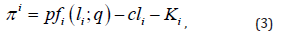
Wherep refers to the price of crop and c is the price of fertilizer input1. Per parcel fixed costs i K differ between technologies and consist of labour, fuel, seed, and capital costs. Society cares about the climate and other environmental impacts of crop production. Agricultural GHG emissions (expressed as CO2 equivalents) come from four sources:manufacturing and transporting of fertilizers, cultivation practices (ploughing, harrowing, planting, pesticide application, harvest, etc.), grain drying and finally, emissions from soil. Emissions from manufacturing and transporting fertilizers Eim , are linear in fertilizer application Eim==ε li, from cultivation practices Eif, are constant per hectare and depend on the chosen cultivation technology (for instance, no-till entail less tractor work and thus fuel use). Emissions from soil, denoted by Eis depend partly on the chosen tillage method and amount of fertilizer application. The former emerge from decomposing organic material (CO2emissions) and the latter from nitrification and denitrification caused by soil bacteria (NE2O emissions). Thus, soil emissions as the sum of the two components are,
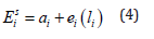
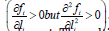
where ai refers to technology specific soil emissions and ei(li) denotes N2O emissions from soils due to nitrogen fertilizer use (the first and second derivatives are positive).
We express the total emissions asEi =Eim+Eif+Eis . Let denote the social damages from climate emissions. In each field parcel of quality q nutrient runoff depends on the use of fertilizer and exogenous variables such as soil type (denoted by θ) as follows:

Thus, nutrient runoff strictly increases with fertilizer application. Nutrient runoff damage is denoted by a convex damage function

It is not necessary that all current arable land is devoted to cultivation under climate mitigation or water quality policy. We assume that a part of arable land may be allocated to sequester carbon or reduce nutrient runoff through establishment of green set-asides or some field parcels may even be afforested.When a given field parcel is allocated to long-term green set-aside, the depleted carbon content of soil starts gradually increase via sequestration. This process is finite in terms of both quantity and time of soil carbon sequestration.
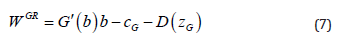
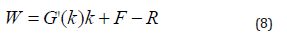
We use the annualized average value of sequestered carbon per year and denote byb . We denote the marginal benefits from carbon sequestration that is from emissions abated by G’(b) > 0 and green set-aside maintenance and establishmentcosts by G c .For forestry we focus on carbon sequestration of afforested land over one rotation period and denote the amount by k, so that the marginal climate benefits are G’(k) > 0, the present annualized value of harvested timber is F and establishment costs R. Finally, (constant) runoff from green set-aside is denoted by G z . In afforested lands nutrient runoff reduces to the level of natural background runoff. As neither of these land uses is fertilized, nutrient runoff is constant. Social net returns to these land-use forms can be given as,
All parts of the policy model are now established. The challenge of the social planner is to design a policy that implements the social optimum.
1In Finland farmers need also to dry the grain; this is a special feature of northern rainfed countries, such as Scandinavian countries. We skip this in the theoretical analysis, because it would only work as a reduction of effective output price. We account grain drying in the empirical application.
Optimal policy design
The economic problem of the social planner is to choose the use of inputs, tillage method and land allocation so as to maximize the social welfare from agriculture when either GHG emissions or nutrient runoff or both are considered. The social welfare function is defined as follows,
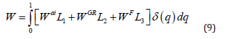
Subject to L1 + L2 + L3 = 1 , that this, the shares of land uses should equal unity.
The first-order conditions governing the interior solution of the social optimum, where all land is allocated between the three uses, can be expressed as,
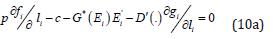
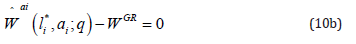
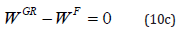
Equation (10a) determines the fertilizer intensity per parcel as a function of land quality, market parameters and external effects. Equations (10b) and (10c) determine the critical land qualities governing land allocation between the cultivated area, green set-aside and afforestation. The solution depends also on tillage method: for each field parcel that tillage method is chosen which produces highest social returns. Finally, note that tillage method related soil emissions are present in net returns to cultivation and carbon sequestered in green set-aside and afforestation.
Farmer’s private solution can easily be extracted from the first-order conditions (10a)-(10c) by setting all external effects equal to zero. Thus, the choice of fertilizer use would reduce to


The climate tax on fertilizer use is uniform, that is, the tax rate is the same over all land qualities. This tax fixes the private fertilizer intensity to the socially optimal level and at the same time ensures that the farmer chooses the socially preferable tillage method. The rest of the policy instruments are needed to establish the socially optimal land allocation.
Equation (11) indicates that information requirements now extend up to soil emissions and soil carbon sequestration, as they are need to set the soil emissions tax and carbon sequestration subsidies at optimal level.We discuss next how the policy focus on climate damage versus water quality damage impacts policy design. Suppose first that water quality policies focus on the same measures as climate policies, then the society uses a Pigouvian tax on fertilizer and a lump sum tax on nutrient runoff from green set aside and afforestation. The Pigouvian fertilizer tax rate is defined by τ* = D′(.) g'l , and it is differentiated over soil types and qualities.
The features of fertilizer tax are well-established [1,13]. Whether the tax rate is uniform or differentiated by soil quality depends on the properties of nutrient runoff. If nutrient runoff is independent of soil quality, the optimal tax is uniform but it is differentiated if runoff properties differ between different qualities see [1]for general discussion on how heterogeneous land quality impacts differentiation of policy instruments). The lump sum nutrient runoff tax on green set-aside and afforestation reflects nutrient runoff from these land uses, which is very low relative to nutrient runoff from cultivated land. The nutrient runoff tax on afforestation is the average annual present value of the runoff damage (see [26] for nutrient runoff and design of forest-specific instruments to reduce nutrient runoff).
When the society addresses both externalities simultaneously, accounting for the co-benefits tends to increase the fertilizer tax but leaves the soil emission tax unchanged. Furthermore, it decreases the size of climate subsidy on green set-aside (due to minor constant runoff damage) and leaves the subsidy on afforestation unchanged (see Appendix).

The optimal fertilizer tax rate increases relative to climate policy only and is no longer uniform. Tax on soil emissions remain the same but the net subsidy for afforestation and green set-aside may be positive or negative depending on relative value of climate benefit from carbon sequestration and nutrient runoff damage. We examine empirically how much the inclusion of nutrient runoff damages would reinforce the impacts of climate policies, what is the relative role of land allocation versus productive inputs and how the instruments perform with respect to fiscal effects, that is, from government net tax revenue viewpoint.
Parametric Model
We now introduce the empirical counterpart of the theoretical model and employ it to examine the role of productive input and land allocation in reducing nutrient loads and GHG emissions. The model is calibrated to agricultural, economic and environmental data collected from Southern Finland. Spring barley (Hordeum vulgare) is selected as a representative crop, because it is the most common crop covering about half of the field parcels under crop cultivation [26] Table 1. The soil type under cultivation is assumed to be one of the three most common soil types; clay, loam and organic soil. Clay soils cover over half of the cropland area in Finland, organic about 14% and loam 35% [27].
Table 1: Fertilizer intensity under private and social optima (kg/ha).

Crop cultivation
Farmers use a compound fertilizer that contains nitrogen and phosphorus in fixed proportions and target yield response to nitrogen application. Mitscherlich nitrogen response function is employed for spring barley.
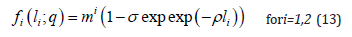
where liis nitrogen application rate and m, σ and ρare parameters. Yields are usually slightly higher on conventionally tilled fields compared to no-till. Yields also depend on soil type:clay soils provide highest and loam soil lowest yields. As for soil qualities, the maximum yields are about 21% higher on high quality soil and about 11% lower on low quality soil compared to the mean yields. Appendix I, Table A1 collects the production parameters regarding Mitscherlich nitrogen response function and costs and prices related to barley production.
Appendix I: Derivation of tax instruments
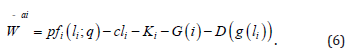
We derive optimal tax rates given the socially optimal solution in equations (9)-(10c). We levy the instruments on fertilizer application and soil emissions and derive conditions which lead to the social optimum. Farmer’s profits from crop production under the nitrogen tax τ targeting both climate emissions and nutrient runoff and soil emissions tax T are
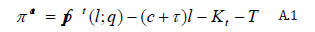
In the presence of carbon subsidies, s, private profits from green set-aside and forestry, respectively, are given by,
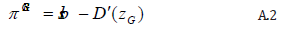
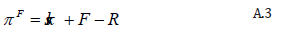
The farmer chooses fertilizer application, tillage method and land allocation between alternative land-use forms so as to maximize total profits from land:
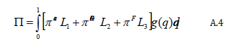
subject to L1 + L2 + L3 = 1 that this, the shares of land uses should equal unity
The first-order conditions governing the interior solution of the social optimum, where all land is allocated between the three uses, can be expressed as,
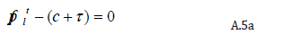
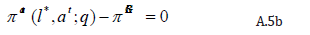
As the system is recursive, the optimal emission tax on fertilizer application can be determined by setting conditions (10a) and A.5a equal and determining τ that produces the equality:

The optimal tax on the use of fertilizers: τ = G′(E)E'+D'(.) glt and if only climate impacts are accounted for the tax rate is τ = G′(E)E' Under this condition the private fertilizer intensity coincides with the socially optimal one.
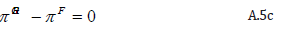
The tax on soil emissions can be solved by setting the private indirect profits equal to indirect social returns and solving for the tax, which gives T* = G′(E)as This guarantees that all externalities are internalized and the private choice of cultivation technology coincides with the social choice. Comparing next the social returns to green set aside with the private one in a similar manner shows that they are identical by choosing the net subsidy rate as
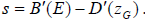
Table A1: Production factors for crop cultivation (Ervola et al. 2012)..

* Harvesting and crop drying are contracted out ** The difference between the technologies.
Greenhouse gas emissions
For greenhouse gas emissions under different fertilizer intensities we refer directly to the result Table 2 (for a general discussion on GHG emissions, see [3]. Emissions include both soil emissions and emissions from input use including nitrous oxide, carbon dioxide and methane fluxes from the whole life cycle of crop production, excluding the emissions from crop consumption. All the soil types are sources of nitrous oxide emissions while organic soils are also a substantial source of carbon dioxide. Methane fluxes are either very small or even negative [28,29].
Table 2: Greenhouse gas emissions under private and social optima (kg CO2 eq./ha/year).

* Harvesting and crop drying are contracted out ** The difference between the technologies.
According to Finnish empirical studies, carbon dioxide emission fluxes from agricultural soils are either similar or even greater under no-till compared to conventional tillage see Table 2. Recently, empirical studies have shown that it is likely that no-till and conventional tillage do not differ in terms of their impact on soil net carbon content, but the carbon is accumulated to different parts of the soil layer keeping the net carbon balance more or less equal [30,31]. Afforestation and green fallow are both suggested to be good options to increase soil carbon. [32] have studied the carbon cycle during 80 years on an afforested land area on mineral soils and noted that the accumulation continues but at a decreasing rate to the end of the rotation.
Figure 1:Carbon dioxide fluxes on mineral and organic afforested soils..

Lohila et al.[33] examined 30 year old forest on organic soil that was previously under crop cultivation. Figure 1 describes the evolvement of carbon in mineral soils and organic soils drawing on[32,33]. To describe the beginning of the forest rotation on organic soil in Figure 1, we use data from bare fallow [34]. Emissions from a newly afforested land are considerably higher during the first years due to increased soil respiration on both mineral and organic soils [35]. However, for organic soils the beginning of the rotation period is often more difficult and the soil is bare or with only light vegetation for a longer period of time. We assume that the forest is cut at the end of the rotation (after 80 years) and again replanted. Forest management practices affect its carbon balance and to keep the carbon lost in minimum forest cutting and renewal practices should disturb soil as little as possible [35](Figure 1).
More detailed information on GHG emissions from afforestation and green fallow are reported in Appendix I. Table A2. As noted, mineral soils are sinks of carbon in both land use options, while organic soils are either a source (green fallow) or a minor sink (afforested). To be able to account the damage (benefit) from climate emissions (carbon sequestration) we need to change the GHG fluxes into monetary values and for this we employ the estimate of marginal damage of carbon dioxide emissions 0.02€/ kg CO2 eq. This value is derived from the study by [36]on marginal damage costs of carbon dioxide emissions.
Table 2A: Parameters for nutrient runoff from crop cultivation

*Varies in terms of the soil type, quality and policy.
Nutrient runoff
We include both nitrogen and phosphorus runoff and in the case of phosphorus we account both dissolved reactive phosphorus (DRP) and particulate phosphorus (PP). Because in compound fertilizer (NPK) the three main nutrients are in fixed proportions, nitrogen fertilizer intensity determines also the amount of phosphorus used. Part of this phosphorus is taken up by the crop, while the rest accumulates and builds up soil P. The concentration of dissolved phosphorus in surface runoff depends linearly on the easily soluble soil P, and the runoff of particulate phosphorus depends on soil erosion and the P content of eroded soil material.
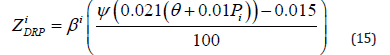
Drawing on Finnish field experiment studies we assume that 1kg increase in soil phosphorus reserve increases the soil P status (i.e., ammonium acetate-extractable P) by 0.01mg/l soil. [37] estimated the following linear equation between soil P and the concentration of dissolved phosphorus (DRP) in runoff: water solubleP in runoff (mg/l) = 0.021*soil_P (mg/l soil)-0.015 (mg/l).
The surface runoff of potentially bioavailable particulate phosphorus is approximated from the rate of soil loss and the concentration of potentially bioavailable phosphorus in eroded soil material as follows: potentially bioavailable particulate phosphorus PP (mg/kg eroded soil) = 250* ln (soil_P (mg/l soil))-150
[37]. Thus, the parametric description of surface phosphorus runoff is given by
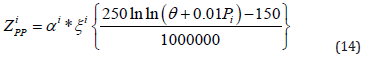
In equation (14) for particulate phosphorus, ζi is erosion rate (kg/ha), θ the amount of soil phosphorus (mg/l). Soil_P is fixed at 10.6mg/l, which is the average for Finnish FADN farms situated in southern and south-western Finland Myyrä et al. [39].In equation (15) ψ is the amount of surface runoff (mm/ha). Piis in both equations the phosphorus application rate (kg/ha). Runoff and erosion differ within no-till and conventional tillage, but the amount of soil phosphorus is the same for both tillage methods. Tillage method specific factors, αi and βi, describe the distinctive characters of the no-till and conventional tillage,
For nitrogen runoff we use [40] nitrogen runoff function calibrated to the Finnish agriculture by [24].
Where Z1i= nitrogen runoff at fertilizer intensity level li, kg/ha, =nitrogen runoff at average nitrogen application, 0 b < 0 and 1 b > 0 are constants and i l = nitrogen fertilization in relation to the normal fertilizer intensity for the crop, 0.5 ≤N≤1.5. This runoff function represents nitrogen runoff generated by a nitrogen application rate of i l per hectare and the parameter reflects differences in tillage methods.
Optimal Use of Inputs and Land Allocation
We now derive numerically the optimal policy design that requires first solving the private and social optima and based on those the policy instruments. We then examine the relative contribution of input choices and land allocation on nutrient runoff and GHG emissions.
Use of inputs, GHG emissions and nutrient runoff
We report the privately and socially optimal levels of nitrogen fertiliser application in Table 1. Given the complexity of our heterogeneous land quality model, the results are presented in combinations of soil types and qualities and for both cultivation technologies. We indicate the policy focus in parentheses.The difference between private and socially optimal fertilizer intensity depends on the policy focus on environmental impacts. If the focus is on nutrient runoff the difference is on average around 20kg/ha for conventional tillage and around 10kg/ha for no-till.
When policy focuses on CO2 equivalent emissions the socially optimal nitrogen application intensity is about 10kg lower than privately optimal. Considering both GHG emissions and nutrient runoff further reduces socially optimal fertilizer applications. While no-till entails lower fertilizer intensity than conventional tillage when focus is only on GHG emissions, it has higher intensity when nutrient runoff damages are taken into account. The reason lies in the fact that no-till results in much lower nutrient runoff than conventional tillage.2
GHG emissions as a primary policy goal and as cobenefits
Table 2 presents the GHG emissions from cultivation practices under different policy focuses. For all policies, we report CO2eq. emissions (CO2, N2O and CH4) from crop cultivation practices anddenote itby E. In a separate row we report the soil emissions under both technologies (for a closer description of data, see Ervola et al. [3]. Soil emissions differ greatly between soil types but only marginally between qualities. Soil emissions from organic soils are more than ten times higher than those from clay soils and several times of those from loam soils. Differences between technologies are minor relative to differences in soils.
Soil emissions make almost 50% of all emissions on clay soils and over 50% on loam soils. In organic soils these emissions are five times higher than those from cultivation practices. These figures provide an important lesson: there is a need to develop new crop production systems (for instance, crop rotations based on legumes and perennial crops) that strengthen carbon sequestration and reduce soil emissions. The middle rows of Table 2 (runoff and CO2equivalent emissions) provide the cases for the analysis of co-benefits produced. With two exceptions on low quality soils, nutrient runoff policy results in GHG emissions that are smaller than those under climate policy only, since the socially optimal input use intensity is lower under the former policy.
Thus, climate co-benefits from water quality policy are significant.Policy addressing both climate and water quality objectives results in the lowest GHG emissions as socially optimal input use intensities are further decreased. Finally, GHG emissions from cultivation practices are lower for no-till than conventional tillage due to lower use of fossil fuels.
Nitrogen runoff as a primary policy goal and as co-benefits
Table A3:Parameters for afforestation and forestry

2 To be more specific, no-till reduces considerably both nitrogen and particulate phosphorus runoff relative to conventional tillage. The well-known drawback is that no-till increases dissolved phosphorus runoff. Lankoski et al. (2006) find in their case that when the reduction of nitrogen and particulate phosphorus are taken into account and valued in monetary terms, benefits from their reductions outperform the costs of increases in dissolved phosphorus.
Table 3 presents the nitrogen runoff (N) kg/ha (for nitrogen and phosphorus runoff expressed as nitrogen equivalents see Appendix I: Table A3). The nitrogen runoff is between 15 and 20kg/ha under conventional tillage and 7.5 to 10kg/ha under no-till.
Table 3:Private optimum vs. alternative social optima: Nitrogen runoff from crop cultivation kg/ha/year.

These results show that in the case of no-till cultivation climate policy internalising CO2-eq damage also achieves socially optimal nitrogen runoff in almost all cases, while in the case of conventional tillage water quality objectives are only partially met with climate policy. Overall, however, climate policy results in significant water quality co-benefits.
Deviation of water quality and GHG damages from the social optimum
Figure 2:Nitrogen application, nutrient runoff damage, GHG damage and social welfare under climate and water quality policies relative to a policy targeting both environmental externalities.

Figure 2 illustrates how much a policy focusing only on GHG damage or nutrient runoff damage deviates from the first-best policy, which internalises both externalities. The first-best benchmark is represented by the 0% line in the figure and we report deviations in terms of nitrogen application, water quality and GHG damages and social welfare. If only nutrient runoff damage is internalised, then the divergence from the socially optimal benchmark is not very large. Nutrient runoff damage differs by 3% and GHG damage by 5%, and the social welfare estimate is only 1% lower than in the first-best solution that internalises both externalities.
If policy targets only GHG damage, then the difference to the social optimum internalising both externalities is much larger especially regarding GHG damage (-18%) and social welfare (-26%). Thus, in terms of both runoff and GHG damage, water quality policy performs much better than climate policy.The deviation of the two second-best policies from the benchmark stem primarily from the use of nitrogen fertilizer, which remains at much higher level when the policy targets only GHG emissions but is only slightly higher than the benchmark when policy targets only nutrient runoff.
The difference in nitrogen application, in turn, is created by the facts that valuation of water quality is much higher than that of GHG damage and that the relative role of nitrogen application causing nitrogen runoff is higher than its role with regard to GHG emissions. So, ultimately these outcomes are explained by both valuation estimates and properties of nitrogen runoff and GHG emissions functions.Results reported in Tables 1-3 determine the private profits and social returns to crop cultivation for all soil types and each land quality. Before reporting the respective land use choices, we examine how competitive long-term green setaside and afforestation are privately and socially in comparison to crop cultivation.
Land allocation between crop production, green setaside and afforestation
Long-term green set-aside produces climate benefits by sequestering carbon back to arable soils. Afforestation does the same thing via tree growth but unlike green set-aside, it also means a reduction in the arable land area. Annual costs of green set-aside are quite modest, 34€/ha/year (including both the establishment and management costs). Afforested land produces harvest revenue but for the first rotation period the annualized present value of net returns is modest, about 48€/ha/year Ollikainen&Lankoski[41]. We report the carbon sequestration, private profits and the social returns for green set-aside and afforestation in Table 4.
Figures reported in Table 4 represent net impact, that is, carbon sequestered minus nitrous oxide emissions. Mineral soils (clay and loam) are an important sink of carbon and provide positive climate net benefits. For afforestation we bundled clay and loam soils together, as data is reported on mineral soils as an aggregate. Organic soils sequester carbon but only slightly and the nitrous oxide emissions exceed sequestration by a wide margin making the net emissions positive but definitely lower than under cultivation. The lower part of Table 4 shows that private profits from green setaside are negative (in the absence of support payments) and private revenue from afforestation is much lower than the social returns. Social returns to green set-aside are positive in loam soils but not in other soil types.
Table 4:Carbon sequestration, private profits and social returns: afforestation and green fallow.

*Negative values indicate net carbon sequestration and positive values emission fluxes.
Privately and Socially Optimal Land Allocation
The privately and socially optimal land allocation between all three land-use forms is presented in Table 5. In crop production these returns reflect the most profitable cultivation technology. The details are allocated to Appendix I, Table A1. We report soil types and qualities used in crop production with the tillage method (notill or conventional tillage) and use acronym AF for afforestation. We denote social returns by W and report the figures in parentheses.
No-till cultivation is more profitable both privately and socially, than conventional tillage mainly due to lower production costs. The only exception to the choice of tillage method can be found on the highest quality loam soils, where conventional tillage is chosen instead of no-till for the case where policy focus is solely on CO2 equivalents. Irrespective of soil types, soil qualities matter a lot. Under the social optima related to climate change (W2 and W3), the minimum and mean qualities in loam and organic soils are allocated to afforestation. Green set-aside turns out never be optimal due to its low carbon sequestration relative to forestry.
Relative impact of input use intensity versus land allocation
We next present our results in a form that facilitates the analysis of the role of input use intensity and land allocation. We decompose the relative impacts of input use and land allocation as follows. The benchmark is the privately optimal use of inputs and land allocation reported in Tables 1&5 respectively. The benchmark contains also CO2-eq GHG emissions and nitrogen runoff under privately optimal solution, which are reported in Tables 2 & 3. We compare the privately optimal benchmark with Policy 3 (W3) that internalises both externalities.
From Table 5 one can find out that there are five cases, where the optimal Policy 3 induces a change in land allocation, that is, a shift from the private optimum to the socially desired one.In all these cases land is allocated from no-till cultivation to afforestation. For these five cases Table 6 illustrates the relative impact of input use intensity versus land allocation in reducing nitrogen runoff and CO2-eq. GHG emissions.
Table 5:Carbon sequestration, private profits and social returns: afforestation and green fallow.

Table 6:Carbon sequestration, private profits and social returns: afforestation and green fallow.

The intensity effect is determined so that we compare GHG emissions and nitrogen runoff for no-till under the privately optimal solution and under Policy 3 (W3) without allowing for a change in land allocation. Thus intensity effect shows the impact of input use intensity on emissions and runoff between privately optimal solution and Policy 3 (W3).
The land allocation effect is determined by the difference in GHG emissions and nitrogen runoff between privately optimal notill and socially optimal (Policy 3) afforestation that is, now we do not allow a shift to the socially optimal fertilizer intensity(Table 6).
Results clearly demonstrate that land allocation effect is many times stronger than intensity effect. For nitrogen runoff, intensity effect results only in 11-13 % reduction while land allocation produces 77-78% of the reduction in nutrient runoff. For GHG emissions, the intensity effect produces 2-3% reduction and only in one case 7% reduction. The land allocation effect has impacts through soil carbon sequestration and emission reductions range from 75% to 235%.Hence, we conclude that reduction potential is very asymmetric, land allocation taking care of most.
Hence, we can conclude that the land allocation effect dominates the intensity effect, or to put it in terms of the theoretical model the extensive margin impact dominates the intensive margin impact. This finding has important implications for both climate and water quality policies. In the case of climate policy, the role of land allocation effect is especially strong on clay and loam soils, where its dominance is reinforced through soil carbon sequestration. As a result, land allocation change from cultivation (with no-till) to afforestation makes these soil types a sink of GHG emissions instead of source.
Afforesting low productivity lands provides one important source for sinks and helps to promote Paris Climate Accord. Given that inputs and land allocation have such an asymmetric impacts on the environment; it is also interesting to ask if this asymmetry translates to the fiscal properties of tax/subsidy instruments. This will be discussed in the next section.
Policy Instrument Design for Climate and Water Quality Objectives
Optimal policy instruments
We next determine the set of Pigouvian policy instruments that internalize climate and water quality damages resulting from private solution. The instrument set must induce the private farmers to choose optimally fertilizer intensity and tillage method over all soil types and qualities, and to allocate land optimally between crop production and carbon sequestration. We also estimate the fiscal impacts of the suggested set of taxes and subsidies. Given that many policy instruments are differentiated, we make an additional analysis to see, how much accounting for policy related transaction costs would impact the fiscal properties of the system.
Table 7:Optimal fertilizer tax rate (€/kg N and %).

We start with the Pigouvian tax on fertilizer and report in Table 7 the optimal tax rates for both tillage methods over the soil types and qualities. We denote the tax rate by τ. It is expressed in terms of €/kg and parentheses provide its percent value relative to fertilizer price.If only CO2 equivalent emissions are accounted for, the optimal tax is a uniform 24 cents per kg of nitrogen fertilizer over all soil types, qualities and tillage methods. If only water quality damage is internalised, then the optimal tax rate is doubled for conventional tillage but for no-till the difference to CO2 equivalent tax is very small. The optimal tax rates increase when both climate and water quality damages are internalised simultaneously. Note however, that the increase is less than the sum of tax rate under separate policies showing that there are synergies between both targets.
In this case the optimal tax rates increase up to 75 cents/kg N (58%) for conventional tillage and 51 cents (39%) for no-till. Tax rates differ between soil types, qualities and tillage methods. Internalisation of water quality damage only leads to tax rates that are non-uniform and vary between soil types, qualities and tillage methods.The tax rates are lower for no-till, because no-till entails significantly lower nutrient runoff than conventional tillage. We next focus on the tax on soil emissions related to tillage methods (which were reported in Table 2).
The optimal soil emissions tax is a lump sum tax, which is obtained by multiplying the amount of (fixed) soil emissions with the marginal damage from climate emissions, that is 0.02€/kg CO2 eq. Recall, the soil emissions range from 760kg CO2eq./ha/year in clay soils to 11544kg CO2 eq./ha/year in organic soils. Thus, this tax would hit most severely organic soils: tax would be € 230.9/ ha in organic soils but only €15.2/ha in clay soils. Thus, the tax on organic soils is really significant when compared to the profitability of cultivation in organic soils (see private profits of cultivation in Annex Table A1).
Finally, a consistent policy mix must entail a net subsidy on green set-aside and afforestation as alternative carbon sequestering land use options. This subsidy covers the net climate benefits from green set-aside and afforestation and depends on soil type, as well as, whether CO2 or CO2eq. emissions are accounted for. We report the tax/subsidy rates in Table 8. Figures with minus sign denote subsidies and those without it are taxes. For afforestation we have combined clay and loam soils together as mineral soils, because GHG measurement in forestry does not separate between them.
Table 8:Tax-subsidy payments on green set-aside and afforestation, €/ha/year.

Starting with green set-aside, organic soils continue to be a source of GHG emissions, and consequently they are taxed. Despite this fact, tax creates incentives for land-use. To see this, just note that while the tax on soil emissions in cultivated land was 231 euros, it is now less than half of it. Green set-side is subsidized in clay and loam soils and for loam soils subsidies are rather high, close to 100 euros/ha. Actually, green set-aside in loam competes very well with afforestation in mineral soils. Interestingly, organic soils turn out to be a challenge for afforestation, too, and when CO2eq. emissions are accounted for, they are subject to taxation instead of subsidization.
Using this set of three policy instruments establishes the social optimum through the choices of private farmers. We provided the proof for this assertion in the theoretical part and the proof by our numerical calculation is shown in Appendix I, Table A1. This table shows that the choices concerning fertilizer use, tillage method and land allocation are identical over soil types and qualities.
Fiscal effects of policy designs with co-benefits
We finally provide estimates on the fiscal effects of the socially optimal policy and the two second-best policies defined by equations (11) and (12). We calculate the impacts of optimal instruments on the government net revenue, while also considering public sector transaction costs (administrative costs) for different policy designs. For this purpose, we multiply the per hectare tax or subsidy payments by the respective shares of total arable land area in each land quality in Finland. The total crop production area in 2009 was about 1.2 million hectares. This land area is distributed between soil types and qualities as follows: clay soils contain 51% of the land area, loam 35% and organic soils 14%. The best qualities in each soil type are assumed to cover 25%, mean qualities 50% and low qualities 25%.
Public sector transaction costs for design, implementation, monitoring and enforcement may differ greatly between different policies and thus affect the overall social welfare effects as well as fiscal aspects of the given policy instrument. The policy-related transaction costs (PRTCs) belong to the class of institutional transaction costs. Accounting for PRTCs is important for several reasons:
a) It improves comparison among and screening of alternative policy instruments,
b) It can help the effective design and implementation of policy instruments to achieve policy objectives,
c) It improves the evaluation of policy instruments, and
d) It helps track budgetary costs of policy instruments over their whole life cycle McCann et al. [42]. Despite the importance of PRTCs for policy choice, PRTCs have seldom been formally included in environmental policy making OECD [43]. Moreover, there are only a few studies that provide empirical estimates of PRTCs of environmental policy instruments.
Here we follow Ollikainen [2] who assess policy-related transaction costs associated with the main agricultural and agrienvironmental policy instruments in Finland. On the basis of this study we estimated the following public sector transaction costs for the policy instruments (as a share of total payment transfer or tax revenue):
(i) Uniform fertilizer tax 9.4%,
(ii) Differentiated fertilizer tax 27.3%,
(iii) Soil emissions tax 17.5%, and
(iv) Subsidy for afforestation and green set-aside 9.4%. We use these figures to provide transaction costs adjusted government tax revenues.
Table 9:Tax-subsidy payments on green set-aside and afforestation, €/ha/year.

W1 = Water quality policy,
W2 = Climate policy, and
W3 = Climate and water policy combined.
Note: Soil qualities are allocated to min 25%, mean 50% and max 25%. Minus sign indicates net subsidy for afforestation.
Table 9 collects the tax revenues and subsidy payments and sums up the net revenue on each policy scheme. It demonstrates how complex the sources for government tax revenue can be: soil qualities, soil types and land allocation provide a variable tax base that is a function of the tax rates-a feature not quite often present in ordinary tax policy.
Starting with minimum soil qualities and water quality policy 1 (W1) all soil types are cultivated with no-till and total fertilizer tax revenue is 23.7M€. Since water quality policy is implemented through differentiated fertilizer tax, which entails relatively high PRTCs, the net tax revenue adjusted with PRTCs is 21.4M€. Note that policy 1 does not entail soil emission tax (denoted by xx in Table 6). Climate policy (W2) collects tax revenue of about 9 million euros (as a sum of the fertilizer tax and tax on soil emissions) from clay soils while loam soils receive net subsidy for afforestation and organic soils pay net tax[44-47]. Overall climate policy results in slightly positive net tax revenue. If water quality aspects are included (W3), the land is shifted to afforestation for which the subsidy payments are about 16M€ euros per year.
In the mean land quality, all clay soils are under cultivation but loam and organic soils are allocated to afforestation when climate policy belongs to the policy package. In these qualities, all policies bring more tax revenues than provide subsidy payments but the range is large starting from five million euros and raising up to 18 million euros. Finally, all best quality lands are allocated to cultivation, so that they bring tax revenue only[48-50]. Even though taxes are quite high on the best quality lands, cultivation is so profitable that taxation does not thread its profitability.
The last column of the Table 9 reports government net tax revenues that are adjusted to reflect public sector transaction costs related to different policy instruments. Results show that when differentiated fertilizer tax is part of the policy (W1 and W3) then consideration of PRTCs significantly reduces net tax revenue from a given policy scenario, while in the case of uniform fertilizer tax (W2) this reduction is clearly lower. Table 10 sums up net tax revenues of each policy over the soil types and qualities and results in aggregate net tax revenues per year.
Table 10 shows that net tax revenues differ depending on the scope of policy. If transaction costs are omitted the lowest net tax revenue results from climate policy, because nutrient runoff damage tax is not collected and there are subsidy payments for afforestation. Water quality policy brings tax revenues from cultivated land and there are no subsidy payments for afforestation and thus this policy results in the highest net tax revenue[51]. The second highest net tax revenue is raised when both climate and water quality are addressed.
Table 10:Aggregate net tax revenue under each policy scenario.

Consideration of PRTCs changes the net tax revenue ranking of policies (last column of Table 10). Now climate policy (W2) results in the second highest net tax revenues, while combined policy (W3) results in the lowest net tax revenues. Policies targeting water quality have relatively strong reduction in the net tax revenue due to the requirement to implement differentiated fertilizer tax that entails relatively high PRTCs.
Conclusion
Many agri-environmental practices, such as reduced fertilizer use or establishment of green set-asides, may have simultaneous positive effects on multiple environmental goods. If these environmental co-benefits are large, then they increase the social benefit of a given policy instrument. We focused on water quality and GHG emissions and examined how climate and water quality policy instruments affect both their primary target emission and co-benefit emissions. We showed that if only water quality damage is internalised then the divergence from social optimum where both damages are internalised is not very large, while if only GHG emissions damage is internalised then the difference to the social optimum internalising both externalities is much larger[52]. Thus, climate co-benefits from water quality policy are significant. Consequently, a coordinated policy design for water quality and climate policy is warranted in order to improve economic efficiency of government policy interventions.
If the change in nutrient runoff and GHG emissions is decomposed to input use and land allocation effects, changes in the land use have a much stronger effect on reducing water quality and GHG emission damages than changes in input use. This suggests that the extensive margin impact (land allocation) dominates intensive margin impact (intensity of input use). This has implications for policies, as discussed later. Does the asymmetry between input and land allocation effects translate to fiscal properties of policy instruments if policy-related transactions costs (PRTCs) are taken into account? Policy scenario focusing on water quality results in the highest net tax revenues, because it does not include subsidies (unlike climate policies).
Accounting for PRTCs reduces considerably net tax revenue and changes the ranking of policies. This reveals the obvious trade-off between precision (differentiated taxations) and transaction costs. Transaction costs are lower for land-use based measures, which is easy to monitor. This is an argument for the use of simpler secondbest instruments.Our analysis has important bearing for designing second-best policies. Consider, for instance, the implementation of the Paris Climate Accord and France’s 4‰ initiative.
Our analysis suggests that allocating low quality lands to carbon sequestration will promote most efficiently climate mitigation with lots of water quality co-benefits. Moreover, observable land use based measures, such as green set-aside or afforestation, are much easier to enforce (compliance monitoring and verification) than input use measures, such as reduced fertiliser application. The challenge in land-use changing policy instruments is the fiscal burdenss. This challenge can be reduced by linking actions for carbon sequestration to emerging mechanisms of carbon compensations and carbon neutrality.
Equally interesting implication is that if governments run only water or climate policy, the deviation from the first-best is smaller for water policy. This should be kept in mind in the preparation of new Common Agricultural Policy (CAP) reform. The reform will expectedly give more role for climate targets, and this is of utmost importance. But this should not lead to abandoning water quality policy targets. Therefore, climate policies should promote those measures that also promote water quality improvements. Coherence between climate and water quality targets must be kept in mind.
All in all, there is still much to do on the way towards climatesmart agriculture that is managed in coherence with water quality targets.
References
- Lichtenberg E (2002) Agriculture and the environment, In: Gardner B, Rausser G (Eds.), Handbook of Agricultural Economics. Agriculture and its extenal linkages. Amsterdam, North Holland, Netherlands, 2(1): 1249-1313.
- Lankoski J, Lichtenberg E, Ollikainen M (2008) Point-nonpoint effluent trading with spatial heterogeneity. American Journal of Agricultural Economics 90(4): 1044-1058.
- Ervola A, Lankoski J, Ollikainen M, Mikkola H (2012) Mitigation options and policies in agricultural sector: a theoretical model and application. Food Economics 1-15.
- Lankoski J, Ollikainen M (2011) Biofuel policies and the environment: Do climate benefits warrant increased production from biofuel feedstocks? Ecological Economics 70(4): 676-687.
- Smith P, Martino D, Cai Z, Gwary D, Janzen H, et al. (2008) Greenhouse gas mitigation in agriculture. Philosophical Transactions of the Royal Society Biological Science 363(1492): 789-813.
- Bangsund D, Leistritz L (2008) Review of literature on economics and policy of carbon sequestration in agricultural soils. Management of Environmental Quality: An International Journal 19(1): 85-99.
- Paustian K, Antle J, Sheehan J, Paul E (2006) Agricultures Role in Greenhouse Gas Mitigation. Prepared for the Pew Center on Global Climate Change.
- Braden J, Segerson K (1988) Information problems in the design of nonpoint-source pollution policy. Theory, Modeling and Experience in the Management of Nonpoint-Source Pollution 1-36.
- Griffin R, Bromley D (1982) Agricultural Runoff as a Nonpoint Externality: A Theoretical Development. American Agricultural Economics 64 (3): 547-552.
- Shortle JS, Dunn JW (1986) The relative efficiency of agricultural source water pollution control policies. American Journal of Agricultural Economics 68 (3): 668-677.
- Segerson K (1988) Uncertainty and Incentives for Nonpoint Pollution Control. Journal of Environmental Economics and Management 15(1): 87-98.
- Xepapadeas A (1995) Observability and choice of instrument mix in the control of externalities. Journal of Public Economics 56 (3): 485-498.
- Horan RD, Shortle JS (2005) When Two Wrongs Make a Right: Second Best Point Nonpoint Trading. American Journal of Agricultural Economics 87(2): 340-352.
- Lichtenberg E (1989) Land quality, irrigation development and cropping patterns in the Northern High Plains. American journal of Agricultural Economics 71(1): 187-194.
- Lankoski J, Ollikainen M (2003) Agri-environmental externalities: a framework for designing targeted policies. European Review of Agricultural Economics 30(1): 51-75.
- Parks PJ, Hardie IW (1995) Least-cost forest carbon reserves: costeffective subsidies to convert agricultural land to forests. Land Economics 71(1): 122-136.
- Stavins RN (1999) The costs of carbon sequestration: a revealedpreference approach. The American Economic Review 89 (4): 994-1009.
- Pautsch GR, Kurkalova LA, Babcock BA, Kling CL (2001) The Efficiency of Sequestering Carbon in Agricultural Soils. Contemporary Economic Policy 19(2): 123-134.
- Antle J, Capalbo S, Mooney S, Elliott E, Paustian K (2001) Economic Analysis of Agricultural Soil Carbon Sequestration: An Integrated Assessment Approach. Journal of Western Agricultural Economics Association 26(2): 344-367.
- McCarl B, Schneider U (2000) US agricultures role in a greenhouse gas emission mitigation world: An economic perspective. Review of Agricultural Economics 22(1): 134-159.
- Weersink A, Joseph S, Kay B, Turvey C (2003) An economic analysis of the potential influence of carbon credits on farm management practices. Current Agriculture, Food & Resource (4): 50-60.
- Metcalf G (2007) A proposal for a U.S carbon tax swap. An equitable tax reform to address global climate change. The Hamilton project. The Brookings institution’s Discussion paper, Russia.
- Aldy J, Eduardo L, Parry WH (2008) A tax-based approach to slowing global climate change. Resources for the future 1-34.
- Pérez Domínguez I, Britz W, Holm Mueller K (2009) Trading schemes for greenhouse gas emissions from European agriculture: A comparative analysis based on different implementation options. Review of Agricultural and Environmental Studies 90(3): 287-308.
- Ancev T (2011) Policy Considerations for Mandating Agriculture in a Greenhouse Gas Emissions Trading Scheme. Applied Economic Perspectives and Policy 33(1): 99-115.
- Lankoski J, Ollikainen M, Uusitalo P (2006) No-till technology: benefits to farmers and the environment? Theoretical analysis and application to Finnish agriculture. European Review of Agricultural Economics 33(2): 193-221.
- Miettinen JM, Ollikainen L, Finer H, Koivusalo A, Lauren (2012) Diffuse load management with biodiversity co-benefits: the optimal rotation age and buffer zone size. Forest Science 58: 342-352.
- Tike (2010) Yearbook of Farm Statistics, Information Centre of the Ministry of Agriculture and Forestry.
- Puustinen M, Turtola E, Kukkonen M, Koskiaho J, Linjama J, et al. (2010) VIHMA-A tool for allocation of measures to control erosion and nutrient loading from Finnish agricultural catchments. Agriculture, Ecosystems & Environment 138(3-4): 306-317.
- Regina K, Alakukku L (2010) Greenhouse gas fluxes in varying soils types under conventional and no-tillage practices. Soil & Tillage Research 109(2): 144-152.
- Lohila A, Aurela M, Tuovinen JP, Laurila T (2004) Annual CO2 exchange of a peat field growing spring barley or perennial forage grass. Journal of Geophysical Research 109(D18).
- Baker J, Ochsner T, Venterea R, Griffis T (2007) Tillage and soil carbon sequestration-What do we really know? Agriculture, Ecosystems & Environment 118: 1-5.
- Luo Z, Wamg E, Sun O (2010) Can no-tillage stimulate carbon sequestration in agricultural soils? A meta-analysis of paired experiments. Agriculture, Ecosystems & Environment 139(1-2): 224- 231.
- Kolari P, Pumpanen J, Rannik U, Ilvesniemi H, Hari P (2004) Carbon balance of different aged Scots pine forests in Southern Finland. Global Change Biology 10(7): 1106-1119.
- Lohila A, Laurila T, Aro L, Tuovinen JP, Laine J (2007) Carbon dioxide exchange above a 30-year-old Scots pine plantation established on organic-soil cropland. Boreal Environment Research 12: 141-157.
- Maljanen M, Sigurdsson B, Gudmundsson J, Óskarsson H, Huttunen J, et al. (2010) Greenhouse gas balances of managed peatlands in the Nordic countries-present knowledge and gaps. Bioscience 7(9): 2711-2738.
- Jandl R, Lindner M, Vesterdal L, Bauwens B, Baritz R, et al. (2007) How strongly can forest management influence soil carbon sequestration? Geoderma 137(3-4): 253-268.
- Tol RSJ (2005) The marginal damage costs of carbon dioxide emissions: an assessment of the uncertainties. Energy Policy 33(16): 2064-2074.
- Uusitalo R, Jansson H (2002) Dissolved reactive phosphorus in runoff assessed by soil extraction with and acetate buffer. Agricultural and Food Science in Finland 11(4): 343-353.
- Uusitalo R (2004) Potential bioavailability of particulate phosphorus in runoff from arable clayey soils. Agri food Research Reports 53, Doctoral Dissertation, MTT Agri food Research, Finland.
- Myyrä S, Ketola E, Yli-Halla M, Pietola K (2005) Land improvements under land tenure insecurity: the case of pH and phosphate in Finland. Land Economics 81: 557-569.
- Simmelsgaard S (1991) Estimation of nitrogen leakage functionsnitrogen leakage as a function of nitrogen applications for different crops on sand and clay soils. In: Rude S (Ed), Agricultural Economics Research Institute, 217. Nitrogen fertilizers in Danish agriculture-present and future application and leaching. Report 62, Institute of Agricultural Economics. Copenhagen: Institute of Agricultural Economics (in Danish): 135-150.
- Ollikainen M, Lankoski J (2009) Multifunctionality: Environment versus Rural Viability in Social Optima. Journal of Rural Development 32(2): 31-57.
- McCann L, Colby B, Easter KM, Kasterine A, Kuperan KV (2005) Transaction costmeasurement for evaluating environmental policies. Ecological Economics 52(1): 527-542.
- OECD (2007) The Implementation Costs of Agricultural Policies. OECD, Paris, Italy.
- Berg S, Lindholm EL (2005) Energy use and environmental impacts of forest operations in Sweden. Journal of Cleaner Production 13: 33-42.
- EEA (2011) Greenhouse gas emission trends and projections in Europe 2011. European Environment Agency. Tracking progress towards Kyoto and 2020 targets.
- IPCC (2007) Contribution of Working Group III to the Fourth Assessment Report of the Intergovernmental Panel on Climate Change. Metz B, Davidson OR, Bosch PR, Dave R, Meyer LA (Eds.), Cambridge University Press, United Kingdom and New York.
- Mäkinen T, Soimakallio S, Paappanen T, Pahkala K, Mikkola H (2006) Liikenteen biopolttoaineiden ja peltoenergian kasvihuonekaasutaseet ja uudet liiketoimintakonseptit. VTT tiedotteita research notes 2357 Abstract in English.
- Mäkiranta P, Hytönen J, Aro L, Maljanen M, Pihlajatie M, et al. (2007) Soil greenhouse gas emissions from afforested organic soil croplands and cutaway peat lands. Boreal environmental research 12: 159-175.
- Ollikainen M, Lankoski J, Nuutinen S (2008) Policy-related transaction costs of agricultural policies in Finland. Agricultural and Food Science 17(3): 193-209.
- Plantinga A, Wu J (2003) Co-benefits from carbon sequestration in forests: Evaluating reductions in agricultural externalities from an afforestation policy in Wisconsin. Land Economics 79(1): 74-85.
- Rørstad PK, Vatn A, Kvakkestad V (2007) Why do transaction costs of agricultural policies vary? Agricultural Economics 36 (1): 1-11
- Vermont B, De Cara S (2010) How costly is mitigation of non-CO2 greenhouse gas emissions from agriculture? A meta-analysis. Ecological Economics 69(7): 1373-1386.
© 2018 Markku Ollikainen. This is an open access article distributed under the terms of the Creative Commons Attribution License , which permits unrestricted use, distribution, and build upon your work non-commercially.
Editor In Chief


.jpg)


Signup for Newsletter

Quick Links
 Editorial Board Registrations
 Submit your Article
 Refer a Friend
 Advertise With Us
Our Recent Edition

.jpg)


Top Editors


.jpg)


.bmp)
.jpg)
.png)
.jpg)


.jpg)


.png)

.png)


.png)


Financial Support

Sponsors

Latest e-Books

Latest Video

 a Creative Commons Attribution 4.0 International License. Based on a work at www.crimsonpublishers.com.
Best viewed in
a Creative Commons Attribution 4.0 International License. Based on a work at www.crimsonpublishers.com.
Best viewed in