
- About Us
- Information
-

The Author ensures that the research has been conducted responsibly and ethically with adherence to all relevant regulations. read more..
- For Authors
- For Reviewer
- Manuscript Guidelines
- Membership
- Publication Ethics
-
- Journals
- Reprints
- e-Books
- Videos
- Policies
- Contact Us
 COVID-19
- Submissions


Full Text
Evolutions in Mechanical Engineering
Internal Combustion Engine Modeling Framework in Simulink: Combustion Modeling
Bradley Thompson and Hwan-Sik Yoon*
Department of Mechanical Engineering, The University of Alabama, USA
*Corresponding author:Hwan-Sik Yoon, Department of Mechanical Engineering, The University of Alabama, USA
Submission: March 04, 2022;Published: April 29, 2022

ISSN 2640-9690 Volume4 Issue2
Abstract
An internal combustion engine modeling framework has been developed in the MATLAB/Simulink environment to allow engine component blocks to be connected in a physically representative manner to reduce the model build time. Each component block, derived from physical laws, interacts with other blocks according to block connection. In this series paper, detailed combustion modeling is presented among several engine subsystems. In the engine modeling framework, combustion is represented by a spherical flame propagating from the spark plug, and the burn rate is correlated to combustion chamber geometry, laminar flame speed, and turbulence. To accurately predict the burn rate, the quasi-dimensional model requires tuning. The combustion model has been computationally validated in a previous study and will be experimentally validated with real engine test data in the next series paper.
Keywords:Internal combustion Engine; Engine modeling; Engine simulation; Combustion modeling
Introduction
High-fidelity engine simulation enables the prediction of performance gains obtained from changes in engine design or control strategies. Based on the simulation results, engine design can be optimized for fuel economy, power, and emissions without relying on extensive experimental data. With the recent advancement in the modeling and simulation methodologies along with computing power, it is possible to run extensive engine simulations with high accuracy these days [1-5].
Among several different approaches in engine simulation, a reduced dimension modeling approach (1D manifold flow and 0D cylinder) is used in many commercial software packages due to its balanced compromise between simulation accuracy and computational time [6- 9]. From a modeling standpoint, the 1D flow model predicts mass transfer into and out of the cylinder during intake and exhaust, while the cylinder combustion model predicts piston force and engine torque eventually. Combustion models vary in complexity and can be categorized as burn rate fit or semi-predictive models. Burn rate fit models match the combustion burn rate based on cylinder pressure measurements [10,11]. Because the burn rate depends on several factors, the models are only appropriate near the tested operating conditions. Semi-predictive combustion models, on the other hand, model combustion at a wide range of operating conditions [12,13]. Unlike the burn rate fit model, semi-predictive models include tuning parameters independent of the operating conditions, and thus employed in the current modeling framework.
Most of the currently available 1D physics-based engine simulation tools are not compatible with or directly implemented in the prevalent MATLAB/Simulink simulation environment. To resolve this deficiency, a high-fidelity physics-based engine simulation modeling framework has been developed in MATLAB/Simulink recently [14-16]. Among the various components in the framework, modeling details of the 1D intake and exhaust flow dynamics were presented in a previous publication [17] based on the work of Blair [18]. As a continued effort, the detailed combustion modeling approach employed in the Simulink-based modeling framework is presented in this series paper. Since the accuracy of the developed tool was numerically validated in the previous paper by comparing the simulation results of a Simulink-based model and commercial software for a single-cylinder pressure change, those who are interested in the model validation are referred to the previous paper [15]. The combustion and dynamics models presented in this paper as well as 1D flow model presented in the previous paper are experimentally validated with a Mazda SKYACTIV®-G 2.0L engine in the next series paper.
Crank Dynamics
A reciprocating piston engine utilizes a slider-crank mechanism to convert linear piston forces into rotational torque. Referring to the engine slider-crank mechanism shown in Figure 1, the piston position xp has a nonlinear relationship with the crank angle θc that depends on the stroke Ls and rod length Lr. The distance from the crank axis to the wristpin s can be determined by the law of sine and cosine since the crank rotational radius a is half the cylinder stroke. Assuming the piston origin to be at the piston Top Dead Center (TDC) and xp = Ls at Bottom Dead Center (BDC), the piston position can be calculated as
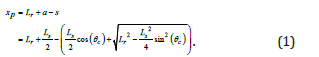
Similar to position, the instantaneous piston speed Sp has a direct relationship with the crank velocity ωc. Differentiating Eq. (1) with respect to time, yields
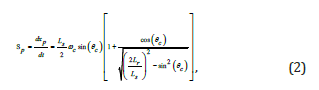
where the crank velocity ωc is defined as
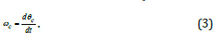
Frequently, the mean piston speed Sp is an important parameter for discussing engine characteristics and predicting the cylinder heat transfer coefficient. Averaging Eq. (2) over a crank revolution results in
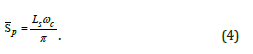
Figure 1:Engine slider-crank geometry.

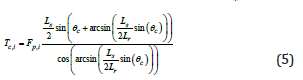
Referring to Figure 1, the cylinder pressure produces a resultant force Fp that axially loads the connecting rod. The connecting rod then applies vertical and horizontal forces to the crankshaft, creating a rotational torque. Neglecting the connecting rod friction and inertial effects, the ith cylinder torque Tc,i can be calculated as/
If the sum of the cylinder torques exceeds the load torque Tload, the crankshaft will accelerate, and if Tload exceeds the sum of cylinder torques, the crankshaft will decelerate. Applying Newton’s second law for rotational motion, the crank acceleration αc is governed by
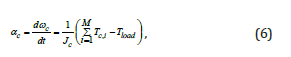
where Jc is the moment of inertia of the rotating assembly and M is the number of cylinders. Because the piston and rod masses are neglected, all inertial effects are lumped into Jc.
Cylinder Conservation Laws
The cylinder is modeled as an open thermodynamic system, where the pressure inside the cylinder is assumed uniform, neglecting 3D flow field effects. If the combustion chamber is treated as a homogeneous single volume, the cylinder model is referred to as a single-zone “zero-dimensional” (0D) model. The volume temperature and pressure are derived from the conservation of mass and energy. If the combustion chamber is split into burned and unburned zones (two-zone model), the model is sometimes referred to as “quasi-dimensional.” The flame propagates spherically from the spark location until quenched by the cylinder walls, thus requiring consideration of the chamber geometry. Both zones have the same pressure but different temperatures. While a single-zone model is typically used for modeling the gas exchange process and compression, a single-zone or two-zone approach can be used during combustion. Conservation of mass and energy for the two models are discussed in this section.
Single-zone and gas exchange period
Figure 2: Diagram of engine cylinder control volume.

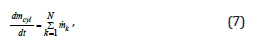
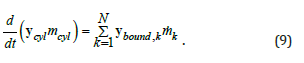
Cylinder temperature Tcyl and pressure pcyl vary according to the conservation of mass and energy. Referring to Figure 2, the mass flows across the boundary through N intake and exhaust ports. Assuming that the flow into the cylinder is positive, the law of conservation of mass states that
where k indexes intake and exhaust valves. During intake and exhaust, the rate of change of cylinder mass fractions ycyl depends on the flow direction. The kth boundary mass fractions ybound,k are defined as
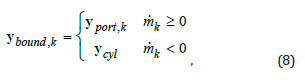
where yport,k is the mass fractions in the kth port. Applying the law of conservation of mass for each gas species during intake and exhaust gas exchange results in the following:
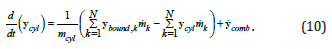
For a single-zone combustion model, the rate of change of mass fractions in the cylinder y comb is determined by a burned gas profile. By combining the combustion rate contribution and the conservation of mass relationship in Eq. (9), the cylinder gas species is governed by
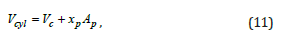
Thermodynamic states are derived from the gas mass in the cylinder mcyl, cylinder volume Vcyl, and internal energy Ecyl. Referring to Figure 2, the instantaneous cylinder volume changes with piston displacement xp according to
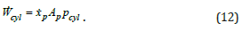
where Ap is the piston area and Vc is the clearance volume. During expansion, the cylinder volume increases, producing work. During compression, work is applied to the control volume. The work transfer rate out of the cylinder volume is the product of piston force and velocity:
According to the first law of thermodynamics, work, flow, and heat transfer across the control volume boundaries shown in Figure 2 govern the rate of change of internal energy Ecyl. Applying the first law of thermodynamics leads to
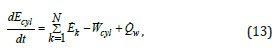
where the kth energy flow rate Ek is determined by the 1D flow model and Ecyl can be defined in terms of specific internal energy or enthalpy as
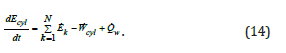
Note that Eq. (13) does not include combustion heat addition because the enthalpies and energies are expressed relative to the same datum.
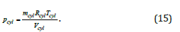
Cylinder pressure pcyl and temperature Tcyl must be derived from the volume Vcyl, mass mcyl, and internal energy Ecyl. For an ideal gas, the internal energy Ecyl is a function of temperature only, which means that Tcyl can be calculated from Ecyl and the internal energy lookup table. Using the cylinder temperature, the ideal gas law leads to
In a real gas law, the internal energy Ecyl becomes an implicit function of pressure and temperature, and the cylinder pressure and temperature must be calculated iteratively.
Two-zone combustion model
Figure 3: Diagram of two-zone combustion model.

The conservation laws presented in the previous section define the cylinder states during intake, exhaust, and single-zone combustion. For a more accurate representation of combustion, the burned and unburned gasses can be separated into two distinct volumes-two-zone model. As shown in Figure 3, the two-zone model assumes a uniform cylinder pressure pcyl with separate zone temperatures (Tu and Tb) and mass fractions (yu and yb). Typically, the burned zone is approximated as a partial sphere with the origin at the spark location. Therefore, as combustion progresses, the unburned gases pass through the spherical flame front into the burned zone, consuming the unburned volume.
Physical constraints and conservation laws must be applied to determine the thermodynamic states shown in Figure 3. Assuming no flow through the valves during combustion, the law of conservation of mass provides the relationship
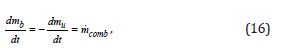
where is the mass burn rate, mb is the burned mass, and mu is the unburned mass. By neglecting heat transfer between the two zones, the conservation of energy applied separately to each control volume yields the following equations:
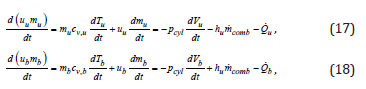
where the specific heat cv is defined as cv = du/dT, the subscript “u” denotes unburned, and the subscript “b” denotes burned. In order to solve for the rate of change of zone temperatures, the volume derivatives must be derived from the ideal gas law. Differentiating the ideal gas equation (defined in Eq. (15) for single zone) for both control volumes leads to
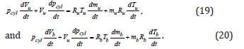
where R is the specific ideal gas constant. Combining Eq. (17) and Eq. (19) and using the specific heat relationship cv,u + Ru = cp,u, the rate of change of the unburned gas temperature Tu becomes
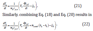
The rate of change of cylinder pressure dpcyl/dt in Eq. (21) and Eq. (22) can be derived from the model constraints. The total cylinder volume defined in Eq. (11) provides the constraints
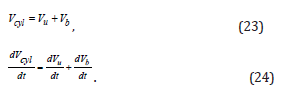
Substituting dVu/dt and dVb/dt from the ideal gas law equations (Eq. (19) and Eq. (20)) into Eq. (24), the following can be concluded:
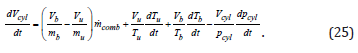
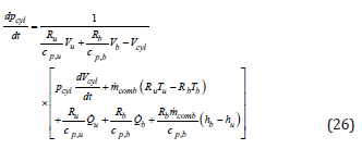
Finally, dpcyl/dt can be derived by substituting Eq. (21) and Eq. (22) into Eq. (25) and rearranging:
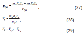
In summary, the rates of change of mu, Tu, and Tb are calculated by Eq. (16), Eq. (21), and Eq. (22), respectively. Therefore, mu and Tb must be initialized at the start of combustion. The initial burned temperature Tb is assumed to be at the adiabatic flame temperature, and to initialize mu, the burned mass mb is derived from the initial spark volume and subtracted from the total cylinder mass. During combustion, gas properties are calculated with the appropriate zone mass fractions and temperature. Cylinder pressure and zone volumes are derived from the ideal gas equations of state:
Cylinder Charge Motion and Turbulence
Turbulence significantly impacts combustion and cylinder heat transfer. To predict turbulence, the cascade concept is frequently employed. Energy from the mean charge motion produces turbulent eddies on the scale of the flow geometry, which break into progressively smaller eddies until the turbulence dissipates at the smallest scale due to viscous shear. During the intake phase, flow through the intake ports produces a mean charge motion, frequently described as swirl and tumble. Intake flow kinetic energy not converted to a swirl or tumble motion produces turbulence. During compression, the rapid increase in density and decay of mean charge motion result in turbulent kinetic energy production. At the same time, the kinetic energy of turbulence at the smallest turbulent length scales dissipates into internal energy. During expansion, little or none of the mean flow remains, and the turbulent kinetic energy continues to dissipate. The turbulent kinetic energy and eddy length scales contribute to the turbulent flame speed.
Mean flow model
Intake port geometry, valve lift, engine speed, and air flow rate all contribute to the mean charge motion. Cylinder flow can also be actively controlled by variable valve lift, valve timing, swirl flap, or tumble flap. Therefore, several factors must be considered in order to estimate cylinder flow across a wide range of operating conditions. Cylinder flow would be best described in three dimensions using the Navier-Stokes equations, but the approach is computationally too expensive. As an alternative, cylinder charge motion is often characterized by angular momentum. The rate of change in angular momentum due to intake flow and turbulence production can be calibrated to match experimental data or CFD simulations [19]. As shown in Figure 4, the angular momentum about the z-axis Lz, referred to as “swirl,” is generated by asymmetric flow through the two intake ports or by the port geometry. Angular momentum about the x-axis Lx, referred to as “tumble,” is generated by the port geometry and the intake port offset from the center of the cylinder. Angular momentum about the y-axis, minor tumble, is ignored. All tumble motion is assumed to be about the x-axis.
Figure 4:Simplified cylinder flow model characterized by swirl angular momentum Lz and tumble angular momentum Lx.

The angular momentum vector describing the cylinder charge motion L is defined as
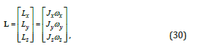
where Jx, Jy, and Jz are the moment of inertias about the three axes, and ωx, ωy, and ωz are the angular velocities about the corresponding axes. The moment of inertias are approximated for a cyinder with diameter B and height xcyl, defined as
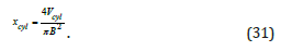
Using a cylinder approximation and assuming the tumble rotation to be centered at xcyl/2 above the piston, the moments of inertia about x and y axes are defined as
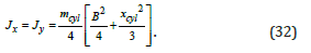
For rotation about the z-axis, the swirl moment of inertia Jz is defined as
Note that Jx and Jy decrease during compression while Jz remains constant. Therefore, without a resistive torque, the tumble velocities ωx and ωy increase while ωz remains constant during compression. The rate of change of angular momentum is determined from the intake flow, exhaust flow, and interaction with the combustion chamber walls. The following assumptions are made to model the swirl Lz and tumble Lx angular momentum [19]:
a. The minor tumble angular momentum Ly is neglected. Lx
accounts for all tumble motions.
b. Tumble and swirl are treated independently.
c. Exhaust backflow has a negligible influence on the charge
motion and turbulence. Therefore, the intake flow is the only driver
of angular momentum.
d. Mass of gas exiting the chamber volume carries angular
momentum
e. Combustion does not affect the mean charge motion.
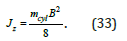
Using the assumptions, the rate of change of tumble angular
momentum Lx can be calculated as
where τx,in is the tumble torque generated from the incoming flow, τx,shr is the tumble resistive torque resulting from shear forces, and ṁex is the total mass flow rate exiting the chamber. In a similar fashion, the rate of change of swirl angular momentum Lz can be calculated as
where τz,in is the swirl torque generated from the incoming flow, and τz,shr is the swirl resistive torque resulting from shear forces. In Eqs. (34) and (35), the first terms represent the charge motion generated by flow through the intake valves, and the second terms represent the fluid shearing forces and wall friction that produce turbulent eddies. The final terms account for the loss of momentum caused by gases exiting the chamber through the intake or exhaust valves. Because little to no angular momentum remains at the start of the exhaust phase, the current cycle has little impact on the swirl and tumble in subsequent cycles. Therefore, Lx and Lz quickly reach a steady state and can be initialized to be Lx=Lz=0. The ability to produce swirl and tumble is frequently quantified by dimensionless swirl and tumble numbers (NS and NT) measured on a steady state flow bench. The ratio between tangential and ideal velocities is one definition of the swirl and tumble numbers published in the literature [20,21]. This definition results in the following relationships between cylinder flow and torque [20]:
where ṁin is the total intake mass flow rate, and uin is the intake flow velocity. NS and NT can be correlated to several factors, involving valve lift, tumble flap angle, swirl flap angle, and pressure drop. Because differences in flow rates between two intake valves affect swirl and tumble, NS and NT cannot be treated independently for each valve. Yun and Lee, for example, measured the swirl and tumble numbers for several combinations of left and right intake valve lifts, producing a two-dimensional lookup table [20]. A similar approach could be used for a swirl or tumble flap. Without charge motion control, NT and NS can be modeled as functions of valve lift only, but the effect of pressure drop can also be included for higher accuracy.
Fluid shear stresses and wall friction degrades the swirl and tumble kinetic energies [22]. The resulting shear torques τz,shr and τx,shr can be determined by integrating the wall friction over the chamber surface and fluid stress over the chamber volume but would require knowledge of the spatial flow field. Grasreiner et al. [19] modeled swirl and tumble flow field as a Taylor-Green vortex and correlated the angular momentum decay using 3D CFD simulations [19]. The authors defined the rate of change of angular momentum due to shear as
Figure 5:Charge motion decay functions Ψx and Ψz derived from 3D Taylor-Green vortex simulations (Adapted from [19])

where Ψdir is the charge motion time decaying function for a given direction, and k is the turbulent kinetic energy. Because the flow structure depends on the chamber geometry, Ψx and Ψz vary with piston displacement and can be adapted to various piston and cylinder head designs. As shown in Figure 5, the tumble decay increases as the piston approaches TDC due to the substantial deformation of the tumble vortex. On the other hand, the swirl vortex shape can be preserved, and the increase in Ψz as the piston approaches TDC can be attributed to increasing frictional losses [19].
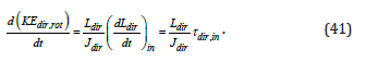
Intake flow kinetic energy is conserved in the form of mean charge motion, turbulent kinetic energy, and internal energy. Rotational kinetic energy in each direction KEdir,rot resulting from Eqs. (34) and (35) is defined as
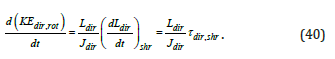
Similarly, the rate of change of rotational kinetic energy due to intake flow is determined by
Turbulence model
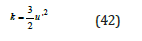
Turbulent flow is irregular and chaotic, consisting of turbulent eddies in a broad range of length scales. The largest length scales are on the order of the flow geometry, and according to Kolmogorov’s theory, energy from the larger eddies is transferred to progressively smaller eddies. The cascade process continues until energy at the smallest length scale dissipates due to viscous forces [23]. Assuming isentropic and homogeneous turbulence, turbulent kinetic energy k is defined from the root-mean-square of the velocity fluctuations u’, such that
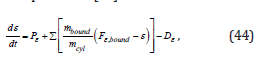
Simplified versions of the k-ε turbulence model have frequently been used in quasi-dimensional combustion models to determine the rate of change of turbulent kinetic energy k and dissipation rate ε. Turbulent kinetic energy and dissipation rate are averaged across the combustion chamber volume. The impact of combustion on turbulence is captured by a modifying factor in the burn rate model discussed later, assuming combustion does not affect turbulence in the unburned zone. Borgnakke et al. described the turbulent kinetic energy balance to have production Pk, diffusion Fk,bound, and dissipation ε terms [24]:/
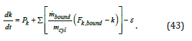
The production term Pk represents the transfer of mean flow energy to turbulent kinetic energy Pk,shr and effects due to rapid changes in density Pk,dens. The diffusion term Fk,bound is treated as a boundary flux, where the fluxes include intake flow Fk,in and fuel injection Fk,inj. The boundary mass flow rate ṁbound only includes flow entering the cylinder because k is defined on a per mass basis. The dissipation rate term ε represents the rate at which the turbulent kinetic energy is destroyed. Similar to the mean charge motion, k has little dependency on the previous cycles and can be initialized as k=0.
Also, similar to turbulent kinetic energy, the dissipation rate is affected by incoming flow, rapid changes in density, and mean flow. One equation k-ε models estimate ε based on the integral length scale-the largest length scale. Two equation k-ε models include an equation for the rate of change of ε derived from the Navier-Stokes equations [25]. Taking a similar form as Eq. (43), the balance equation for ε can be represented [24]:
where Pε is the production, Fε,bound is the boundary fluxes, and Dε is the rate of destruction. Dissipation rate initial conditions depend on the initial k. By setting k=0 initially, ε=0 at the start of simulation. Along with turbulent kinetic energy, eddy length scales are important for predicting the burn rate. In the two-equation k-ε model, the integral length scale lI, which is the largest turbulent length scale, is defined as
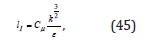
where Cμ is an empirical constant typically suggested to be 0.09. At the Kolmogorov length scale lK, which is the smallest length scale, viscous stresses cause the turbulent kinetic energy to dissipate. The Kolmogorov length scale is defined as
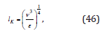
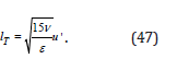
where ν is the kinematic viscosity of the fluid. The Taylor microscale lT, which is smaller than lI and larger than lK, is used to model the eddy burn-up time [26]. The Taylor microscale is defined as/
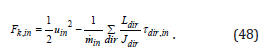
inetic energy crossing the volume boundary contributes to the turbulent kinetic energy and mean charge motion. By subtracting the rate of change of the mean kinetic energy due to intake flow (Eq. 41) from the total intake kinetic energy, the intake turbulent kinetic energy contribution Fk,in can be calculated as
Fuel injection is assumed not to contribute to the mean charge motion. Therefore, all kinetic energy is represented as turbulent kinetic energy. The direct injection contribution Fk,inj is defined as
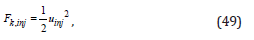
where uinj is the velocity through each injector hole. The effect of exhaust backflow on turbulence is neglected as well.
Intake and direct injection contributions to the dissipation rate are derived assuming the integral length scale of the incoming flow to be proportional to the flow dimension. Using the intake valve lift Lv as the flow dimension and rearranging Eq. (45), the intake dissipation rate contribution Fε,in is defined as
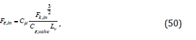
where Cε,valve is a tuning constant. Similarly, the injection dissipation rate term Fε,inj can be written as
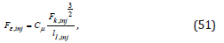
where lI,inj is the integral length scale of the incoming flow. Note that lI,inj represents all injector holes and may not be easily determined from the hole diameters but can be tuned.
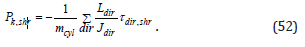
Mean flow kinetic energy KErot,dir is converted to turbulent kinetic energy as a result of wall friction and fluid shear. From Eq. (40), the turbulent kinetic energy production resulting from shear Pk,shr can be written as/
A standard k-ε model relates the turbulence production term Pk,shr to the rate of change of the dissipation rate Pε,shr by
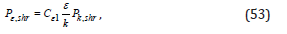
where Cε1 is an empirical constant typically suggested to be 1.44. Similarly, the ε destruction rate Dε is related to ε by
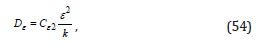
where Cε2 is an empirical constant typically suggested to be 1.92.
In addition to the turbulence produced from the mean charge motion, Borgnakke et al. [24] derived a turbulence production term to account for the effect of compression and expansion [24]. Using the rapid distortion theory, the turbulence produced by rapid changes in density Pk,dens is modeled as
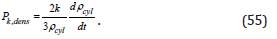
Assuming the turbulent angular momentum to be conserved, the product of u’ and lI remains constant during rapid distortion. Therefore, the following can be concluded [24]:
Spark-Ignition Combustion Burn Ratet
For a typical SI engine, air and fuel are uniformly mixed in the combustion chamber prior to combustion. After the intake valve closes, the piston begins to compress the mixture, and near the end of the compression stroke, the spark plugs initiates combustion. The electric discharge between the spark plug electrodes creates a high-temperature plasma kernel [6]. The kernel then develops into a propagating flame front. At the thin flame sheet, an exothermic chemical reaction occurs, and the unburned mixture is converted to combustion products or “burned gas.” Enclosed by the piston, cylinder wall, and cylinder head, a turbulent flame develops and spreads within the combustion chamber. When the flame front reaches the chamber walls, the flame can no longer propagate.
Several factors influence the rate at which the flame propagates. The reaction mechanism for the combustion of a hydrocarbon involves numerous intermediate reactions that dictate the flame speed. Modeling the reaction from a chemical kinetic perspective would be computationally expensive and would still not necessarily provide an accurate prediction of cylinder pressure. Flame propagation speed also depends on flow within the combustion chamber. Increasing turbulence intensity during combustion increases the flame propagation speed, thus making piston speed, intake geometry, and chamber design important factors. Simplified models tuned with experimental data or CFD simulations must be used to represent complex combustion phenomenon when employing a 0D or quasi-dimensional model. Fitting the burn rate with a Wiebe function, which will be described in the next section, is one way to represent combustion without considering combustion chemistry and turbulence. Because the fitting does not include physics-based representations of combustion, the accuracy will suffer when operating outside the tuned range. A turbulence entrainment model, however, uses laminar flame speed and a turbulence model to predict the burn rate. Although an entrainment model requires tuning, the more predictive approach can better represent combustion outside the operating points used to tune the model.
Wiebe burn rate
The rate of combustion has been observed to gradually increase at the start of combustion, rapidly increase during flame propagation, peak halfway through the combustion process, and rapidly decline during flame termination. Therefore, the mass fraction of burned gas yburn creates an “s-shape” when plotted against the crank angle as shown in Figure 6. Based on experimental observations, the combustion rate is frequently fitted by a Wiebe function in the crank angle domain. The general Wiebe function is defined as
Figure 6:Cylinder pressure and Wiebe mass fraction burned profile.

where θc. is the crank angle, θ0. is the crank angle at the start of combustion, Δθ is the combustion duration, and a and m are fitting parameters. Parameter m defines the shape of the mass fraction burned profile, while a model the combustion efficiency. From Eq. (57), combustion efficiency ηcomb. can be defined as
Parameter a becomes 6.908 for an assumed efficiency of 99.9%. To tune the Wiebe function parameters, cylinder pressures are measured at different engine operating conditions, and the burn mass fraction profile can be derived by energy law analysis [6]. As a result, a, m, and Δθ vary with engine speed and load.
Turbulent entrainment model
Figure 7:Turbulent entrainment model zones with a spherical flame front expanding from the spark location.

The Wiebe mass burn profile provides an accurate estimation of cylinder pressure when simulating combustion at or near the tuning operating conditions. Because the actual burning velocity depends on turbulence and unburned gas composition, however, any changes in cylinder flow or mixture at the start of combustion will produce inaccuracy. For example, altering the valve timing changes the flow velocity into the cylinder, thus affecting turbulence and flame speed. Even spark timing has an effect on the burn rate. Turbulence and flame structure vary with piston position due to changes in pressure, temperature, and cylinder volume, and by moving the start of combustion, the burn rate changes throughout the combustion process. To optimize engine parameters, a more predictive combustion model must be employed to ensure better accuracy over a wide range of operating conditions.
The turbulent entrainment model includes cylinder turbulence, geometry, and composition when predicting the burn rate [26,27]. As depicted in Figure 7, the entrainment model represents combustion in two stages. In the first stage, the unburned mixture is entrained within the turbulent flame front but not consumed. In the second stage, the entrained mass is burned. The rate at which the unburned gasses are entrained by the flame is defined as
where me is the entrained mass, Sf is the turbulent flame speed, and Af is the surface area between unburned and entrained zones. Once entrained, the ignition sites are stretched by turbulent eddies at the Taylor microscale lT until the unburned gasses become fully engulfed by the flame. The mass burn rate ṁb is governed by the eddy burn up time τb and unburned entrained mass:
Tabazynski used the Taylor microscale lT to characterize the spacing between dissipation regions [26]. By adding a tuning constant Cb to Tabazynski’s model, τb is defined as
where SL is the laminar flame speed.
Tabazynski represented the flame speed Sf as the sum of the laminar flame speed SL and the root-mean-square of velocity fluctuations u’ [26]:/
Several additions have been made by researchers to better match experimental observations. Brehob and Newman modeled the flame speed with the following equation [28]:
where rf is the flame radius and Cf and Cdev are tuning constants. During early combustion, turbulence has less impact on the flame speed. The exponential term in Eq. (63) models the transition from laminar to turbulent flame speed. Throughout combustion, the propagating flame impacts turbulence. Different approaches have been used to correct u’ for rapid changes in density. The square root of the density ratio in Eq. (63) accounts for the effect combustion has on turbulence.
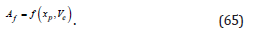
Area Af can be determined from a 3D CAD model or a generic representation of the chamber with the flame front approximated as a sphere centered at the sparkplug. A lookup table for Af can be generated by intersecting a sphere with the combustion chamber geometry (cylinder wall, piston, and cylinder head) at flame radius rf and piston position xp breakpoints. The volume inside the sphere Ve can be determined from the geometry as a function of flame radius rf and piston position xp as well. By integrating flame speed (ṙf=u’+SL), rf can be estimated and then used to determine Ve and Af from lookup tables. However, the model becomes over constrained when deriving rf from the flame speed because Ve, a function of rf, is defined by the two-zone model constraints. Thus, assuming the unburned entrained density to be ρu, the entrained volume Ve is defined as
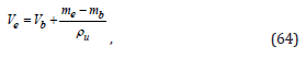
where the burned volume Vb is defined in Eq. (28). Now, Ve can be used as breakpoints for the Af lookup table:
Laminar Flame Speed
Under laminar flow conditions, the reaction layer between the unburned and burned zones (flame front) during premixed combustion propagates in a controlled manner toward the unburned mixture. Based on the observation, premixed combustion is often characterized by the laminar flame speed SL. Detailed reaction mechanisms can be used to predict SL, as described in [29]. Chemical reaction simulations are computationally expensive and may not accurately represent the burn rate. Therefore, SL is typically measured experimentally and fit to a power law.
Several factors influence SL, including pressure, unburned gas temperature Tu, equivalence ratio ϕ, and diluent gas mass fraction ydil (i.e. EGR or burned gas residuals). In order to determine SL for various air-fuel mixtures, Metghalchi and Keck measured the burn rate over a large range of operating conditions and fit SL to the equation [30]:
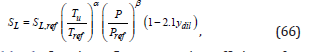
Table 1: Laminar flame speed coefficients for methanol, propane, isooctane, and gasoline.

where Tref = 300K, Pref = 101325 Pa, and α, β, and SL,ref are fuel specific parameters that vary with ϕ. The fit parameters are defined as:/
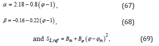
where Bm, Bϕ, and ϕm are fuel specific fitting parameters summarized in Table 1 for various fuels.
Heat Transfer
During combustion and expansion, heat loss due to convection heat transfer lowers the cylinder pressure and therefore usable power. Cylinder wall, cylinder head, and piston are modeled at separate temperatures Twall, Thead, and Tpiston. For a single-zone combustion model, heat transfer Q̇w from the chamber walls to the control volume is defined as
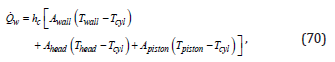
where hc is the heat transfer coefficient and Awall, Ahead, and Apiston are the cylinder wall, head, and piston surface areas exposed to the control volume, respectively. Areas Ahead and Apiston remain constant while Awall varies with xp:
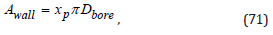
where Dbore is the cylinder bore diameter. For a two-zone combustion model, heat transfer is defined for both zones: unburned Q̇ u and burned Q̇ b heat transfer. Similar to Eq. (70), convection heat transfer for the zones are defined as
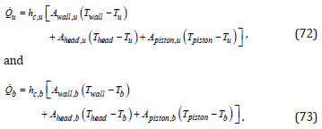
where the surface areas are defined for each zone. Assuming a spherical flame front, each surface area is a function of flame radius and piston displacement. Flow velocity influences the convection heat transfer coefficient hc but is not explicitly available from the cylinder model. To predict cylinder convection heat transfer, Woschni developed a convection correlation based on a spatially averaged cylinder velocity [32]. Woschni suggested that the average gas velocity w in the cylinder should be proportional to the mean piston speed S p , and to account for changes in velocity during combustion and expansion, Woschni included the motoring pressure pm in the correlation. Assuming a polytropic expansion of an ideal gas, the motoring pressure can be estimated from
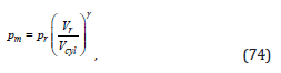
where pr and Vr are the reference pressure and volume taken at the start of combustion. Derived from experimental testing, Woschni published the following correlation for predicting the mean cylinder gas velocity:
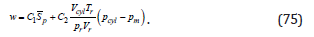
The correlation coefficients C1 and C2 given in Table 2 are adjusted based on specific engine conditions. Valves are open during gas exchange and closed during compression and expansion. As a result, the period can be determined by the flow rate through the valves and the piston speed.
Table 2: Coefficients for Woschni heat transfer correlation [31,32].

With the mean velocity w, Woschni correlated the cylinder Nusselt number to the Reynolds number using the power-law relationship/
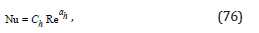
where Ch is a tunable constant and ah=0.8. Woschni used Ch=0.035, but the value could be tuned to fit experimental data. With Dbore as the characteristic length, the heat transfer coefficient can be derived from Eq. (76) as/
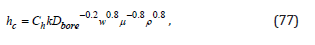
where ρ is the density, k is the thermal conductivity, and μ is the dynamic viscosity of the gas. For the single-zone model, ρ is the cylinder density ρcyl and fluid properties are evaluated at the cylinder temperature Tcyl. For the two-zone model, density and temperatures are taken from the respective zones. Therefore, hc,u ≠ hc,b due to the differences in density and fluid properties.
Conclusion
In this series paper, a detailed combustion modeling approach utilized in a Simulink-based spark-ignition internal combustion engine modeling framework was presented. For the combustion model, both single-zone and two-zone models were explained with an assumption of a spherical flame propagating from the spark plug. The burn rate is correlated to the combustion chamber geometry, laminar flame speed, cylinder charge motion, and turbulence. To accurately predict the burn rate, the quasi-dimensional model requires tuning of several parameters for various empirical models. The overall combustion model was partially validated by comparing a simulation result with commercial software in a previous publication by the authors and will be experimentally validated with real test data obtained from a Mazda SKYACTIV®-G 2.0L engine in the next series paper./
References
- Deppenkemper K, Can OI, Markus E, Markus S, Dirk B, et al. (2018) 1D engine simulation approach for optimizing engine and exhaust aftertreatment thermal management for passenger car diesel engines by means of variable valve train (vvt) applications. SAE Technical Paper.
- Andric J, Schimmel D, Sediako AD, Sjoblom J, Faghani E (2018) Development and calibration of one dimensional engine model for hardware-in-the-loop applications. SAE Technical Paper pp. 8.
- Buhl S, Hain D, Hartmann F, Hasse C (2018) A comparative study of intake and exhaust port modeling strategies for scale-resolving engine simulations. International Journal of Engine Research 19(3): 282-292.
- Onorati A. Montenegro G (2020) 1D and multi-d modeling techniques for ic engine simulation. SAE pp. i-xix.
- Caton JA (2015) An introduction to thermodynamic cycle simulations for internal combustion engines. John Wiley & Sons, New Jersey, USA, pp. 384.
- Heywood JB (2018) Internal combustion engine fundamentals. McGraw-Hill Education, USA.
- Baratta M, Finesso R, Misul D, Spessa E (2015) Comparison between internal and external EGR performance on a heavy duty diesel engine by means of a refined 1D fluid-dynamic engine model. SAE International Journal of Engines 8(5): 1977-1992.
- Alqahtani A, Shokrollahihassanbarough F, Wyszynski ML (2015) Thermodynamic simulation comparison of AVL BOOST and Ricardo WAVE for HCCI and SI engines optimization. Combustion Engines 161(2): 68-72.
- Yontar AA, Doğu Y (2018) Experimental and numerical investigation of effects of CNG and gasoline fuels on engine performance and emissions in a dual sequential spark ignition engine. Energy Sources, Part A: Recovery, Utilization, and Environmental Effects 40(18): 2176-2192.
- Hann S, Palaveev S, Grill M, Veltman M, Bargende M (2020) Predicting the influence of charge air temperature reduction on engine efficiency, ccv and no x-emissions of a large gas engine using a si burn rate model. SAE Technical Paper pp. 18.
- Hann S, Grill M, Bargende M, Altenschmidt F (2020) A quasi-dimensional si burn rate model for predicting the effects of changing fuel, air-fuel-ratio, egr and water injection. SAE Technical Paper pp. 40.
- Tolou S, Vedula RT, Schock H, Zhu G, Sun Y, et al. (2018) Combustion model for a homogeneous turbocharged gasoline direct-injection engine. Journal of engineering for gas turbines and power 140(10): 102804.
- Gefors H (2020) Laminar flame speed modeling for a 1-D hydrogen combustion model, in automotive engineering. Chalmers University of Technology, Gothenburg, Sweden.
- Thompson B, Yoon HS (2014) Development of a high-fidelity 1D physics-based engine simulation model in MATLAB/Simulink, SAE Technical Paper.
- Thompson B, Yoon HS (2015) Continued development of a high-fidelity 1D physics-based engine simulation model in MATLAB/Simulink, SAE Technical Paper.
- Tadros M, Ventura M, Soares CG (2016) Assessment of the performance and the exhaust emissions of a marine diesel engine for different start angles of combustion. Maritime technology and engineering 3: 769-775.
- Thompson B, Yoon HS (2020) Internal combustion engine modeling framework in simulink: gas dynamics modeling. Modelling and Simulation in Engineering 2020: 16.
- Blair GP (1991) An alternative method for the prediction of unsteady gas flow through the internal combustion engine. SAE transactions pp. 28.
- Grasreiner S, Neumann J, Luttermann C, Wensing M, Hasse C, et al. (2014) A quasi-dimensional model of turbulence and global charge motion for spark ignition engines with fully variable valvetrains. International Journal of Engine Research 15(7): 805-816.
- Yun JE, Lee JJ (2000) A study on combine effects between swirl and tumble flow of intake port system in cylinder head. SAE Technical Paper.
- Yadav NK, Saxena MR, Maurya RK (2020) Numerical investigation of in-cylinder tumble/swirl flow on mixing, turbulence and combustion of methane in SI engine. SAE Technical Paper pp. 13.
- Hamid MF, Yusof Idroas M, Saad S, Heng TY, Mat SC, et al. (2020) Numerical investigation of fluid flow and in-cylinder air flow characteristics for higher viscosity fuel applications. Processes 8(4): 439.
- McComb W, May M (2018) The effect of Kolmogorov (1962) scaling on the universality of turbulence energy spectra. arXiv preprint arXiv:1812.09174 pp.10.
- Borgnakke C, Arpaci VS, Tabaczynski RJ (1980) A model for the instantaneous heat transfer and turbulence in a spark ignition engine. SAE Technical Paper pp. 17.
- Nieuwstadt FT, Westerweel J, Boersma BJ (2016) Turbulence: Introduction to theory and applications of turbulent flows. Springer.
- Tabaczynski RJ, Trinker FH, Shannon BA (1980) Further refinement and validation of a turbulent flame propagation model for spark-ignition engines. Combustion and Flame 39(2): 111-121.
- Wang S, Prucka R, Zhu Q, Prucka M, Dourra H (2016) A real-time model for spark ignition engine combustion phasing prediction. SAE International Journal of Engines 9(2): 1180-1190.
- Brehob DD, Newman CE (1992) Monte carlo simulation of cycle by cycle variability. SAE Technical Paper pp.15.
- Ratnak S, Kusaka J, Daisho Y (2015) 3D Simulationson premixed laminar flame propagation of iso-octane/air mixture at elevated pressure and temperature. SAE Technical Paper.
- Metghalchi M, Keck JC (1982) Burning velocities of mixtures of air with methanol, isooctane, and indolene at high pressure and temperature. Combustion and flame 48: 191-210.
- Rhodes DB, Keck JC (1985) Laminar burning speed measurements of indolene-air-diluent mixtures at high pressures and temperatures. SAE Transactions pp.16.
- Woschni G (1967) A universally applicable equation for the instantaneous heat transfer coefficient in the internal combustion engine. SAE Technical paper pp. 19.
© 2022 Hwan-Sik Yoon. This is an open access article distributed under the terms of the Creative Commons Attribution License , which permits unrestricted use, distribution, and build upon your work non-commercially.
Editor In Chief


.jpg)


Signup for Newsletter

Quick Links
 Editorial Board Registrations
 Submit your Article
 Refer a Friend
 Advertise With Us
Our Recent Edition

.jpg)


Top Editors


.jpg)


.bmp)
.jpg)
.png)
.jpg)


.jpg)


.png)

.png)


.png)


Financial Support

Sponsors

Latest e-Books

Latest Video

 a Creative Commons Attribution 4.0 International License. Based on a work at www.crimsonpublishers.com.
Best viewed in
a Creative Commons Attribution 4.0 International License. Based on a work at www.crimsonpublishers.com.
Best viewed in