
- About Us
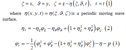
- Information
-

The Author ensures that the research has been conducted responsibly and ethically with adherence to all relevant regulations. read more..
- For Authors
- For Reviewer
- Manuscript Guidelines
- Membership
- Publication Ethics
-
- Journals
- Reprints
- e-Books
- Videos
- Policies
- Contact Us
 COVID-19
- Submissions


Full Text
Examines in Marine Biology & Oceanography
A New Approach to the 2-D Phase- Resolving Modeling of 3-D Surface Waves
Dmitry Chalikov1,2*
1Institute of Oceanology RAS, Russia
2University of Melbourne, Australia
*Corresponding author: Dmitry Chalikov, Institute of Oceanology RAS, 117997 Moscow, Russia. University of Melbourne, VIC 3010, Australia
Submission: March 20, 2023;Published: April 19, 2023

ISSN 2578-031X Volume5 Issue5
Abstract
A new two-dimensional approach to modeling of three-dimensional deep-water potential waves is given. A new approach develops a recent version of the 2-D model for 3-D waves. The 2-D model (A Heuristic Wave Model, HWM) is based on the same two-surface conditions as a 3-D model (A Full Wave Model, FWM), but instead of а 3-D elliptic equation for the velocity potential, its surface projection is used. This equation is not closed, because it contains both the vertical velocity w and its vertical derivative z w . The previous closure scheme was formulated in terms of physical (grid) variables and used some integral parameters. Contrary to that model, a new closure scheme is based on consideration of the vertical structure of Fourier amplitudes for a nonlinear component of the surface velocity w . It is shown that w and its vertical derivatives of the potential at the surface are closely connected. The coefficient in this connection is close to constant. The system of equations of a new HWM includes full surface kinematic and dynamic conditions and an additional diagnostic surface equation for calculation of the surface vertical velocity. Such transformation turns the 3-D formulation for 3-D waves into a 2-D formulation. The applicability of the 2-D model is demonstrated by comparison of the statistical results calculated by FWM and HWM for the identical set of parameters. The main advantage of the 2-D HWM is that it runs about one - two orders faster than a 3-D FWM
Keywords:3-D model of 3-D surface waves; 2-D model of 3-D surface waves; Surface vertical velocity; Input and dissipation of energy; Statistical characteristics of wave field
Introduction
The numerical simulation of surface waves is a special branch of the computational fluid mechanics. In its turn, this section is divided into several directions; most of them refer to the technical fluid mechanics. All the works devoted to study of interaction of waves with various floating and fixed objects, as well as to the behavior of waves in the basins with complex bathymetry and shape of coastline, can be also attributed to this direction (see [1]). As a rule, the models of such kind do not require very high accuracy of solution or a long-term calculation, but their formulation can be extended in order to take into account additional physical effects (for example, turbulence), or even to abandon an assumption of potentiality. Such models are capable of reproducing the strongly non-linear processes. That group also includes the studies of fast local processes, such as wave breaking, interaction of waves with wind and focusing of energy leading to rapid increase in wave height. Free waves are very conservative, i.e., they change their energy over hundreds and thousands of wave periods. In particular, this is true for the processes of nonlinear interactions studied for four wave interactions in [2]. The change of energy due to the interaction of waves with wind and the numerous effects of wave breaking are also very slow. Thus, to correctly reproduce an evolution of wave field, the adiabatic part of the model must be integrated with high accuracy; otherwise, the physical processes will turn out to be distorted by approximation errors. At present, high accuracy can only be achieved for potential formulations. Since the effects of nonlinearity are weak, they can manifest themselves only in the course of a long-term integration over hundreds or thousands of periods of the energy-containing modes. If the scheme is not precise, the cumulative effects of nonlinear interactions (for example, a downshifting process) can be distorted. Fortunately, the potential approximation in most cases turns out to be quite realistic.
From a practical point of view, the most important is the study of the statistical properties of sea waves including the statistics of rare phenomena. For such purposes the 3-D models based on complete potential equations and supplied with the algorithms that describe transformation of wave energy and momentum are most suitable. In such models it is reasonable to use an assumption that the process is periodic in both horizontal directions. It means that the process is considered in a small part of a large area where the horizontal statistical homogeneity is assumed. A simulated area cannot be small, i.e., it should include a wide ensemble of waves of various lengths. On the other hand, the region must be sufficiently small as compared to the spatial scales of transformation of integral characteristics, such as total wave energy. That assumption means that an evolution of wave field is considered in time, not in space. The spatial variation of the statistical characteristics can be estimated by calculations of a fetch based on the phase velocity of a spectrum peak. The assumption of periodicity allows us to use fourier-transform method for solution.
The simplest way is using an adiabatic version of the model, i.e., the simulation of the process with no energy sources or dissipation. To carry out the calculations in such a pure form is difficult due to the computational instability that occurs because of energy accumulation at high wave numbers. To maintain the stability, some sort of dissipation should be introduced to remove an excess energy. The statistical stationarity can be achieved by introducing an appropriate integral energy input that does not change the shape of spectrum. However, the complete stationarity cannot be maintained because of a slow nonlinear transformation of spectrum, widening and shifting of the spectra to low wave numbers (downshifting). Hence, this kind of modeling can be used for investigation of a nonlinear statistical regime of a wave field assigned in the initial condition as a set of linear modes with random phases. These calculations make sense because the transformation of a linear wave field to the nonlinear one occurs relatively fast. The nonlinear features such as sharp crests and gentle troughs, as well as the specific probability distribution for wave height develop over the time of the order of 100-1000 periods of peak wave (depending on the initial nonlinearity of waves).
The simulation of a non-stationary wave regime, in particular, the development of wave field under the action of wind and dissipation is of our main interest. Unfortunately, these studies are severely limited by a lack of understanding of the physical processes, in particular, the interaction of waves with wind and wave breaking. Those processes are the subject of intensive research, but one can hardly say that any reliable parameterization schemes have been offered for any of them. The calculation of the energy input can be based on miles approach [3-6], connecting Fourier coefficients for the surface pressure p and elevation η (see [7]). The modeling of wave evolution is impossible with no parameterization of wave breaking [4]. Considering an exact criterion for the breaking onset is useless, since the numerical instability in such models arises not because of the approach of breaking but because of appearance of large local steepness. An acceptable scheme can be based on a local highly selective diffusion operator with a diffusion coefficient depending on the local curvilinearity of surface [5]. The breaking parametrization algorithms are too simple to be considered as a final solution of the problem, but they are flexible enough to carry out simulation of wave field evolution with reasonable agreement with JONSWAP approximation. Note that the numerical simulation allows reproducing wave transformation within the time and space limits which are orders of magnitude wider than those available in the experiments. Overall, the 3D models supplied with the appropriate physical algorithms are an excellent tool for studying of statistical properties of sea waves. The model should be also used for development and validation of new parameterization schemes. Such models can be adjusted to the phase-resolving simulation of wave regime in small basins with real shape and bathymetry.
A common flaw of all 3-D models is their low performance. For example, our first experiment on development of waves under the influence of wind, performed with a model, (the number of degrees of freedom being of the order of 106 , the number of levels for solving an equation for the potential being equal to 40), took two months of continuous calculations on a computer with speed 2.1GHz. Since it is unacceptable, further steps were taken to develop a more economical scheme. Our main efforts were targeted at reducing the overall dimension of the problem. Both the dynamic and kinematic surface conditions (used as evolutionary equations for elevation η and the surface velocity potential ϕ ) contain the surface vertical velocity w. By contrast with a two-dimensional problem in the conformal coordinates, there is no simple way to calculatew on a 2-D curved surface, so one has to solve in one way or another a complete elliptic 3-D equation for the velocity potential and extract 2-D wfrom the 3-D solution for ϕ . The data on the 3-D ϕ field is no longer required. Note that an equation for ϕ must be solved with high accuracy, so that the solution would take about 95% of computer time and memory. Such approach seems to make no sense. However, it is unlikely that a simple and exact method to compute w without solving an ϕ equation can be ever found. Therefore, it was concluded that an approximate approach was to be found to solve the problem. This method can be based on the analysis of projection of Laplace equation onto a curved surface η (x, y) . An equation obtained is exact, but it contains both the first z ϕ and second vertical derivatives zz ϕ of the velocity potential.
These variables turned out to be closely connected both in the physical (grid) and Fourier spaces. The parameters of this connection were defined with a 3-D Full Wave Model (FWM). The preliminary analysis carried out in terms of Fourier variables did not give any well-defined results. Therefore, a first version of the closure was formulated for grid variables. The approximation used two global variables: the surface variance and the surface curvature variance. Finally, a new model (which we also call Heuristic Wave Model, HWM) included standard dynamic and kinematic boundary conditions and a 2-D diagnostic surface equation for calculation of the surface vertical velocity w(x, y) . The accuracy of a closure method was confirmed by comparison of the results generated by the 3-D and 2-D models running at identical setting and initial conditions [6]. Despite the fact that the new model turned out to be quite suitable for modeling of the statistical regime of a multimode wave surface, we were not fully satisfied with the closure scheme used. The parameters of the scheme turned out to be slightly dependent on global setting of the model. This shortcoming was easy to correct, but in general, the suggested scheme could not be attributed to local schemes. Therefore, it was decided to fall back upon the local parametrization formulated in terms of Fourier coefficients for vertical profiles of the velocity potential near surface. It turned out that the reason for failure of the first of such attempts was insufficient accuracy of calculating the values of a second derivative of the velocity potential near surface. In a new version of the calculations, the number of vertical levels was increased from 30 to 60, while a stretching factor increased from 1.1 to 1.2. The comparison of the numerical values of the derivative with the analytical values showed that the errors of the numerical calculation did not exceed 10−8 (in comparison with norm).
3-D Full Wave Model (FWM)
This model was repeatedly described in previous publications (see for example, [7]), so some details will be omitted here. The equations are written in the non-stationary surface-following nonorthogonal coordinate system:
where ϕ is the surface velocity potential. Laplace equation for Φ at ζ ≤ 0 turns into the equation

The equations (4)-(7) are written in a non-dimensional form using length scale L (2πL is a dimensional period in the horizontal direction) and gravity acceleration The equations (1) and (2) are accepted as the evolutionary equations for elevation and the surface velocity potential ϕ , while a diagnostic equation (4) is solved with the boundary conditions.
Depth is assumed to be large enough to consider a case of deep water for all wave modes.
It is convenient to represent in (4) the velocity potential as a sum of an analytical (‘linear’) component ϕ (Φ) and an arbitrary (‘non-linear’) component ϕ(Φ). The analytical component ϕ satisfies Laplace equation with the known solution:
while the nonlinear component satisfies an equation:
The derivatives of a linear constituent of Φ included in a righthand side of (7) are calculated analytically. The method of solution combines a second-order finite-difference approximation on the stretched staggered vertical grid and a 2-D Fourier-transform method in surfaces ζ = const . An equation (7) in FWM is solved as Poisson equations by TDMA (Tridiagonal Matrix Algorithm) method of prescribed accuracy with iterations over the right-hand side. The number of iterations depends on a maximum of the local surface steepness, and for high steepness it does not exceed three. A 3-D model described above is potentially exact, i.e., it can provide high accuracy with increase of the number of fourier modes and the number of vertical levels. Its only drawback is low performance. Below a scheme is suggested which at a cost of minor loss of accuracy provides a significantly higher speed of calculation.
2-D Heuristic Wave model (HWM)
Since ϕ (0) = 0 , an equation (7) for the velocity potential at ζ = 0 takes the form:
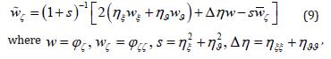
An exact equation (9) contains both the first w ζ ≡ϕ and second wζ ζζ ≡ϕ vertical derivatives of the potential. It was empirically discovered in [6] that those variables are closely connected to each other. Firstly, the dependence between wζ and w was constructed in the physical space. The pairs of local values (w,w ) ζ were generated in multiple numerical experiments with FWM. It was found that the connection between and cannot be formulated in terms of local kinematic and dynamic parameters. Instead, the dependence contained two integral parameters: dispersion of elevation (1/2) σ = η 2 and dispersion of ‘horizontal’ Laplacian ( )1/2 2 elevation. Finally, a formula ( )L w w F ζ= σ σσ was obtained. The approximation for function F is given in [6]. It was demonstrated by comparison of the 2-D and 3-D calculations that such a non-local scheme allows us to reproduce multiple statistical characteristics of wave field with sufficient accuracy. However, this result did not satisfy us, mainly, for aesthetic reasons: The local closure using integral parameters (even despite weak dependence on those parameters and the overall success of application), is very easy to criticize. The previous scheme is inconvenient because it requires tuning when changing integral parameters - (however, it can be done automatically in the course of modeling). The new scheme uses specific features of vertical fourier profiles of the vertical velocity component (Figure 1). The randomly chosen vertical profiles of fourier coefficients given as a function of Φk ,l (ζ ): a - for full values of the velocity potential Φk ,l (ζ ) ; b - for the nonlinear components Φk ,l (ζ ) are given in Fig.1. The values are close to the exponential function of depth ζ . The values of k ,l Φ on the average are two orders of magnitude smaller than the values of k ,l Φ . As seen, Φk ,l (ζ )profiles look very similar to each other, and they have a very simple shape. It is easy to see that the first and second vertical derivatives are connected: with increase of a first derivative (inclination) of , / k l ∂ϕ ∂ζ the second derivative (curvature) (k ,l ) ζζ Φ also grows. The data obtained with very a high resolution over ζ in the vicinity of surface ζ = 0 allows us to suggest that the curves Φk ,l (ζ ) can be approximated by a formula:
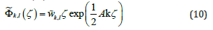
Figure 1:Examples of randomly selected vertical profiles of fourier coefficients: a–full vertical velocity ( ) , 103Φk1 ζ ; b-a nonlinear component of the vertical velocity 7 ( ) 10 Φk ,l ζ .

where w k,l are the values of Fourier coefficients for a nonlinear component of the velocity potential at the surface ζ = 0. Using the relation (10) it is easy to obtain:
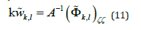
where A is a coefficient which formally can depend on indices k and l. The connection between , wkk,l and (Φk,l)ζζ is shown in (Figure 2).
A coefficient A is defined by comparison of, wkkl and (Φk,l)ζζ values calculated in the course of long-time numerical experiments with 3-D FWM. The resolution was equal to 513× 257 modes and 1024×512knots; the number of levels was to 60, with a stretching coefficient γ =1.20. The depth was equal to4π ; the thickness of the lowest level was equal to 2.0958, while the thickness of an upper level was 0.0017, which provided sufficient accuracy of calculation of derivatives of the velocity potential in the vicinity of surface. The initial conditions for elevation and surface potential were generated with JONSWAP spectrum for the inverse wave age equal to 1 (see [8]), and for the peak wave number equal to 20. The small energy input was compensated by dissipation (see description of the algorithms for input and dissipation in [5]), so the dynamic regime was close to stationary in a statistical sense. The integration was performed for a period Δt =10,000which corresponds to 2,757 peak wave periods. For evaluation of dependence , wkkl and (Φk,l)ζζ as many as 13,052,215 pairs of vertical velocity and its vertical derivatives were used. The averaging was done over (Φk,l)ζζ by 200 bins. An averaged curve is shown in Figure 2 by a thick line overlapped by a straight line:
Figure 2:Dependence of fourier coefficients for the nonlinear surface vertical velocity multiplied by wave number ,wkkl on Fourier coefficients for vertical derivative of the nonlinear vertical velocity (Φk,l)ζζ The line averaged over all the data coincides with the approximating straight line (Eq. (11)); they are shown by a single thick line, while the thin lines indicate dispersion of data. A dashed curve shows the probability distribution for Φζζ normalized by its maximum value.

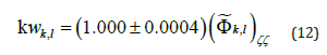
According to (Figure 2), the variables investigated are connected linearly, and the parameter A in (11) is a constant. Thin lines show the scatter of data relative to dependence (12). The scatter grows with an increase of (Φk,l)ζζ, its averaged value being equal to 0.0001. The relation (11) can be used for elimination of wζ from an equation (9), which finally can be represented in terms of Fourier components as follows:

The equation is written in a form convenient for iterations. The upper index corresponds to the number of iterations. The grid variables s, , , , w ξ ϑ ζ η η Δη and Fourier coefficients for , A/k,wkkl variables during iterations remain constant.
A variable w is not included in equations (2), (3) and (9). Therefore, it makes sense to check how accurately the total vertical velocity w = w+ w is calculated. An algorithm based on (13) was inserted in 3-D FWM, which made it possible, when solving the evolutionary problem, to compare the local values of the total vertical velocity calculated by two different methods based on equations (4) and (13). This comparison is shown in (Figure 3) where Fourier coefficients for full vertical velocity calculated with 2-D HWM (W),k,l H and with 3-D FWM (WF k,l) , F k l W are compared. A solid line corresponds to two coinciding curves: one curve is calculated over all data with bins Δw =1.5⋅10−5 and another one is a straight line approximated by the linear function:

The root-mean-square difference between , (W),k,l H and , WF k,l is equal to 10−5 . The number of pairs (WH ,WF )used is equal to 13,052,215. A dashed curve describing probability distribution for , WF k,l shows that maximum values of the vertical velocity fall to the range (−1,+1)⋅10−4 . Figure 3 proves that the surface vertical velocity w (which is a single study object) is calculated in HWM quite satisfactorily.
Figure 3:Comparison of individual values of fourier coefficients for full vertical velocity calculated with 2-D HWM (W),k,l Hand with 3-D FWM ( ) , WF k,l . A thick line shows coinciding of the averaged over bins curve and the approximation [14]. A dashed curve shows probability distribution for , WF k,l.

Comparison of HWM and FWM
A 2-D model developed is not intended (or at least not tested) for direct modeling of individual processes such as wave breaking, but rather for studying of the statistical regime of a multimode wave surface in a region that includes hundreds and thousands of waves for stationary or variable regimes. The reliability of the results reproduced by the model is proved below by comparison of some statistical characteristics obtained by parallel calculations with FWM and HWM at the same initial conditions, identical algorithms for parameterization of the physical processes and the same parameters. The only difference between the models is the way in which the vertical velocity on the surface is calculated: in FWM the values of the vertical velocity are derived from the solution of a 3-D equation for the velocity potential (4), while in HWM the vertical velocity is found by solving a 2-D equation (13).
The calculations over 10,000 time steps were done for the quasi-stationary regime. The parameters of setting are described in Section 3. The data used for estimation of the coefficients in (14) were not used for comparison. The spectra of different characteristics are shown in Figure 4. The 2-D variables were transferred from the rectangular (k,l ) to polar (φ , r ) coordinates (φ is angle, k ,0 r = k is radius) and then summated over the angle. Grey curves illustrate the variability of the spectra. Since the spectra obtained with FWM and HWM models coincide with each other up to the line thickness, they turn out to be indistinguishable in the linear scale. All data show that the spectra for FWM and HWM are very close to each other. The absolute difference between them (shown by dotted curves) is two orders of magnitude less than the compared values.
Figure 4:Spectra of different characteristics obtained in identical runs with FWM and HWM. Grey curves in all panels represent 85 spectra; each of them is obtained by averaging over 10 cases. Thick curves are the spectra averaged over all 850 cases. All thick curves are the superposition of two curves calculated by FWM and HWM. The absolute difference between the averaged spectra is shown by dotted curves. Panel 1 represents the spectrum of elevation η ; 2 is the vertical velocity: two upper curves represent the spectra and difference for full vertical velocity w; two lower curves are the same for a nonlinear component w ; 3 is the spectrum of inclinations ξ η ; 4 is the input energy spectrum; 5 is the loss of energy due to breaking (with an opposite sign); 6 is the spectrum of energy variations due to nonlinear interactions.

Panel 1 shows the spectrum of elevation η . Since the quasistationary regime is supported, the variability of spectrum (grey noise) is small. Panel 2 contains two pairs of curves: two upper curves represent the spectra and difference for full vertical velocity w; two lower curves are the same for a nonlinear component w . The absolute difference between the spectra for FWM and HWM (dotted curves) can be demonstrated only in the logarithmic scale. On the average, the values w are two orders of magnitude larger than the values w , which confirms that w is a small correction of a linear component of the vertical velocity w. The spectrum of inclination (panel 3) and the spectrum of energy input (Panel 4) also confirm high agreement between the data obtained with FWM and HWM. The spectra of energy change due to wave breaking (Panel 5) demonstrate high variability of that process (which seems to be realistic), but the averaged effect of breaking is also similar in both models.
The most interesting is the data on spectrum variations due to the nonlinear interaction (Panel 6). The scatter of the data averaged over 10 cases (grey curves) exceeds the averaged spectra by two orders of magnitude. This effect discovered earlier [7] is explained by small but fast variations of wave mode amplitudes due to the reversible nonlinear interactions. In Hasselmann’s theory those variations are eliminated by averaging over an infinite set of phases, resulting in a residual spectrum change similar to that shown by a thick line for both models. The shape of this curve agrees with the existing views: the energy decreases at a high-frequency slope of wave peak and increases at a low-frequency slope of wave peak. Thus, the process of downshifting arises. This process is not reproduced in our calculations because of an insufficient period of integration. In general, the spectrum data confirms that HWM gives spectral results similar to those obtained with FWM. Below is given a comparison of two models, taking more sensitive characteristics as an example, i.e., the first four moments of the elevation and vertical velocity fields.
The comparison of probability distribution of the first moments for elevation field is given in Figure 5. The curves describing the probability distribution for the moments calculated in HWM and FWM practically coincide. The difference between them is shown in the logarithmic scale with a dotted line. As can be seen, an error in reproducing the moments of elevation field is approximately two orders of magnitude smaller than the typical values of the moments themselves.
Figure 5:The probability distribution for the moments of elevation field: Panel 1-η ; 2-η2 ; 3-η3 ; 4-η4. Black curves calculated with HWM are superimposed with a red curve calculated with FWM. Dotted lines show absolute difference between the moments corresponding to HWM and FWM. The total number of values used for every curve is equal to 519,045,921..

In our opinion, the most important verification of HWM is comparison of the moments of vertical velocity, which in fact is the object of parameterization. This comparison is given in Figure 6. Note that the high-order characteristics presented are extremely sensitive. They are calculated with FWM after solving a complicated 3-D equation (7), while with HWM the same is obtained with a simplified scheme based on a 2-D equation (13) for vertical velocity. The data for the first and second order moments of wcoincides with very high accuracy/. It is seen that for all other moments up to the probability of10−5 −10−4 the agreement is also high. The probability of small values of the third and fourth order moments is underestimated. It is very difficult at present to discuss the reasons for that effect, but it definitely deserves further analysis. Note that comparison of different 3-D models is not very popular, especially for such complicated characteristics as spectra of different variables shown in Figure 4, and the statistical moments in Figures 5&6.
Figure 6:The probability distribution for the moments of vertical velocity field: Panel 1-w; 2-w2 ; 3-w3 ; 4-w4. Red curves are calculated with HWM, while black curves are calculated with FWM. Dotted lines show absolute difference between the moments corresponding to HWM and FWM. The total number of values used for every curve is the same as in (Figure 5).

Discussion
The 3-D models based on the initial potential equations are perfect tools for investigation of physics and statistics of waves. Such models can be used as laboratories for study and parameterization of the physical processes associated with transformation of momentum and energy [5,7]. The only drawback of such models is their high complexity and low computational efficiency. Those shortcomings sometimes result in sheer impossibility to carry out multiple and detailed calculations of evolution of the multimode wave field. Over the past ten years the author has undertaken repeated efforts to speed up the numerical procedure. The proposed schemes were intended to correct obvious clumsiness of the direct approach: A three-dimensional equation for the velocity potential was solved only to calculate the two-dimensional surface velocity field, which was then used for time step with equations for elevation and surface potential. To prevent instability, the vertical velocity must be calculated with high accuracy, i.e., with sufficiently high vertical resolution. To avoid this difficulty, at the stage of calculating the surface velocity it turns out to be convenient to represent it as a sum of a linear component that formally satisfies Laplace equation with the given velocity potential on the surface and as a deviation from it which is equal to zero on the surface [7]. An equation for such deviation can be obtained by projection of Laplace’s equation onto a curved surface. Naturally, a resulting equation, in addition to the vertical velocity, contains its vertical derivative. Thus, the problem of establishing a relationship between those variables (i.e., a closure problem) arises. A first version of the closure scheme [6] was suggested for physical (grid) variables. The scheme included two global coefficients: the averaged potential energy and the averaged curvature. The calculations proved that with a proper choice of those parameters (which are updated during calculation), the model describes the statistical structure and evolution of wave field very well. However, we were not completely satisfied with that result, since the method based on local variables only, seemed more suitable.
A second closure scheme developed in the current paper is based on consideration of vertical profiles of Fourier coefficients for the three-dimensional velocity potential field (Figure 1). It was found that all those profiles in close vicinity of the surface had a shape well described by a simple formula (10). The only coefficient in such formula A =1.07 is determined on the basis of the extensive 3-D results obtained with a high-resolution 3-D model. After closing a surface equation for the velocity potential contains a single unknown variable, i.e., the vertical velocity. An equation [13] is solved by iterations. The comparison of the vertical velocity calculated with 2-D and 3-D models and equations (13) and (7) proves their high agreement (Figure 3). The applicability of a new scheme was proved by comparison of the 1-D spectra for different kinematic and dynamic characteristics calculated by averaging over the entire period of calculations with FWM and HWM (Figure 4). Despite the considerable scatter, all the averaged spectra coincide with the accuracy up to the line thickness. The similar accuracy was demonstrated for very sensitive characteristics, i.e., the first four moments of surface elevation (Figure 5). Even more sophisticated characteristics, i.e., the moments for the surface vertical velocity (which is the object of parameterization) also confirmed satisfactory accuracy (Figure 6). Some deviation of the 2-D results is observed for small values of the 3-d and 4-th moments. In general, the data presented shows that the proposed approach deserves further improvement and testing. In particular, some data shows that a coefficient A in (11) can be a weak function of the spectral steepness of each mode , , kkl Akl where k and A are the modulus of wave number and amplitude.
Acknowledgment
The author would like to thank Mrs. O. Chalikova for her assistance in preparation of the manuscript. This research was supported by RSF (project No. 22-21-00139).
References
- Qingwei M (2010) Advances in numerical simulation of nonlinear water waves. Advances in Coastal and Ocean Engineering 11: 1-700.
- Hasselmann K (1973) On the non-linear energy transfer in a gravity wave spectrum, part 1. General Theory. J Fluid Mech 12(4): 481-500.
- Miles JW (1957) On the generation of surface waves by shear flows. J Fluid Mech 3(2): 185-204.
- Babanin AV (2011) Breaking and dissipation of ocean surface waves. Cambridge University Press, USA, pp. 1-480.
- Chalikov D (2018) Numerical modeling of surface wave development under the action of wind. Ocean Science 14(3): 453-470.
- Chalikov D (2022) A 2D model for 3D periodic deep-water waves. J Mar Sci Eng 10(3): 410.
- Chalikov DV (2016) Numerical modeling of sea waves. 1st (edn), Springer Publishers, USA, pp. 1-330.
- Hasselmann K, Barnett RP, Bouws E, Carlson H, Cartwright DE, et al. (1973) Measurements of wind-wave growth and swell decay during the Joint Sea Wave Project (JONSWAP). Tsch Hydrogh Z Suppl A8(12): 1-95.
© 2023 Dmitry Chalikov. This is an open access article distributed under the terms of the Creative Commons Attribution License , which permits unrestricted use, distribution, and build upon your work non-commercially.
Editor In Chief


.jpg)


Signup for Newsletter

Quick Links
 Editorial Board Registrations
 Submit your Article
 Refer a Friend
 Advertise With Us
Our Recent Edition

.jpg)


Top Editors


.jpg)


.bmp)
.jpg)
.png)
.jpg)


.jpg)


.png)

.png)


.png)


Financial Support

Sponsors

Latest e-Books

Latest Video

 a Creative Commons Attribution 4.0 International License. Based on a work at www.crimsonpublishers.com.
Best viewed in
a Creative Commons Attribution 4.0 International License. Based on a work at www.crimsonpublishers.com.
Best viewed in