
- About Us
- Information
-

The Author ensures that the research has been conducted responsibly and ethically with adherence to all relevant regulations. read more..
- For Authors
- For Reviewer
- Manuscript Guidelines
- Membership
- Publication Ethics
-
- Journals
- Reprints
- e-Books
- Videos
- Policies
- Contact Us
 COVID-19
- Submissions


Full Text
Examines in Marine Biology & Oceanography
The 2-D Heuristic Wave Model for 3-D Waves with a Local Closure Scheme
Dmitry Chalikov1,2*
1Shirshov Institute of Oceanology RAS, Russia
2Department of Infrastructure Engineering, Melbourne School of Engineering, Australia
*Corresponding author: Dmitry Chalikov, Shirshov Institute of Oceanology RAS, 117997 Moscow, Russia and Department of Infrastructure Engineering, Melbourne School of Engineering, Victoria 3010, Australia
Submission: December 02, 2022;Published: January 19, 2023

ISSN 2578-031X Volume5 Issue2
Abstract
A surface equation connecting the vertical velocity and its vertical derivative is used. These variables are well connected in Fourier Space, which allows us to construct the 2-D formulation for modeling of 3-D waves. It leads to the 2-D (surface) formulation for 3-D waves. The comparison of the spectral results generated by 3-D and 2-D models demonstrates their close identity
Keywords: Phase resolving; Wave modeling; 2-D model for 3-D waves; Comparison of 3-D and 2-D modelse
Introduction
A common weak point of all 3-D models is their low performance, since all of them in one way or another resolve the vertical structure of a wave field based on a 3-D equation for the velocity potential. In 3-D model (Full Wave Model (FWM)) [1] this goal was achieved by solving a 3-D equation for the velocity potential. This solution turns out to be unnecessary: to continue the calculations, just the vertical velocity field on the surface is required. Finally, it was found that the solution of the problem can be based on an equation for a nonlinear component of the velocity potential written for the physical surface [2]. This equation is exact but it contains both the first and second derivatives of the velocity potential. It was found that these variables are connected to each other linearly. The coefficients in a linear connection were evaluated by calculations with a high-resolution FWM. Since the method used in 2-D model is based on experimental selection of nondimensional variables and functions, we call this model Heuristic Wave Model (HWM) [2]. The accuracy of a closure method is confirmed by comparison of the results generated by 3-D and 2-D models running at identical setting and initial conditions. The scheme developed in [2] is not universal enough, because the closure of an equation for the vertical velocity uses integral parameters, i.e., those calculated over the entire field. In this paper a local closing in Fourier space is suggested.
Three-Dimensional Phase-Resolving Model
Modeling of 3-D potential waves is based on the system of equations [1]:
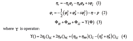
Here ,ξϑ and ζ are curvilinear nonstationary coordinates connected with the Cartesian coordinates ,,:
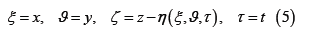
τ is a time; τ η is a time derivative of η ; ξ η and ϑ η are derivatives of η over ξ and ϑ ; Φ is the 3-D velocity potential; ϕ = Φ(ζ = 0) is the 2-D surface velocity potential; ξ ϕ and ζ ϕ are along-surface derivatives over ξ and ϑ ; ζ ϕ is a vertical derivative of the potential on the surface (i.e., the surface vertical velocity); the derivatives of Φare calculated along the surfacesζ = const ; D ξξ ϑϑ ≡η +η is a 2-D Laplacian of elevation; s 1 2 2 ξ ϑ ≡ +η +η ; p is the air pressure on the surface, divided by the water density; η (x, y,t ) =η (ξ ,ϑ,τ ) is a moving periodic wave surface given by Fourier series:
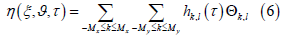
where k and l are the components of the wave number vector k= (k2 + l2) 1/2 ;hk,l (τ) are Fourier amplitudes for elevationsη (ξ ,ϑ,τ ) ; x M and y M are the numbers of modes in the directions ζ andϑ , respectively, while k ,l Θ are the Fourier expansion basic functions. All the variables are scaled with a use of gravity acceleration g and an arbitrary linear scale L .
The 2-D surface boundary conditions (1) and (2) are
considered as evolutionary equations for calculation of η and
the surface fieldϕ . Both equations include a vertical derivative
of the velocity potential ζ ϕ , i.e. the surface vertical velocity w.
For calculation of this variable, we have to solve a 3-D elliptical
equation for volume distribution of the velocity potential for a
surface boundary conditionΦ(ζ = 0) = w . Unfortunately, the values
of ware very sensitive to the details of a numerical scheme. That
is why for exact calculations of the surface vertical derivative of the
potential it is necessary to use a large number of vertical levels and
a stretched grid. An equation (3) is solved as Poisson equation with
recalculations of a 3-D right side. The typical number of iterations is
about 10. Such scheme turned out to be imperfect. The acceleration
was achieved by representing the velocity potential as a sum of two
components: an analytical (‘linear’) component ϕ and an arbitrary
(‘non-linear’) componentϕ : ϕ =ϕ +ϕ , Φ = Φ+Φ
The analytical component ϕ satisfies Laplace equation:
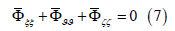
with the known solution:
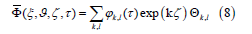
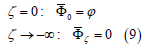
(where k= (k2 + l2) 1/2 , ϕk ,l are Fourier coefficients for the surface potential ϕ atζ = 0 ). The 3-D solution of (7) satisfies the following boundary conditions:
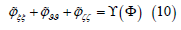
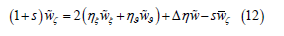
The nonlinear component satisfies an equation:
Thus, Eq. (12) is solved with the boundary conditions:
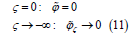
The scheme for solving equation (10) is similar to that for equation (3), but due to simple boundary conditions (11), the number of iterations for the right side is reduced to two, which generally speeds up the solution by 2-3 times.
2-D Equations for 3-D Waves
Anyway, calculation of the 3-D model velocity potential takes about 95% computer time and space. The current paper continues to develop a new approach to the phase-resolving modeling of two-dimensional periodic wave fields. The basic concept of the scheme follows from presentation of the velocity potential as a sum of the linear and nonlinear components suggested in [1]. It was observed in [2] that such approach offers a new way to simplify the calculation by projection of 3-D Poisson equation on the surface:
The equation can be considered as an additional exact surface condition. It contains both the first w ζ ≡ϕ and second wζ ζζ ≡ϕ vertical derivatives of the potential. Thus, the system of equations remains unclosed. It was empirically discovered [2] that those variables are closely connected to each other. There are two possibilities: we can construct dependence between wζ and w in the physical space, i.e., in terms of grid variable. The pairs wζ and w and all the grid parameters were generated in multiple numerical experiments with FWM. It was obtained that the connection between wζ w cannot be formulated in terms of the local kinematic and dynamic parameters. Instead, the dependence contained two integral parameters: dispersion of elevation σ = (η2)1/2 and dispersion of ‘horizontal’ Laplacian σL = (2D of elevation. Finally, the formula ( )L w w F ζ= σ σσ was obtained. An approximation for function F is given in [3]. It was demonstrated in [2] by comparison of the 2-D and 3-D calculations that such a non-local scheme allows to reproduce multiple statistical characteristics of wave field with sufficient accuracy.
Earlier the attempts were made to construct a more flexible local closure scheme not in grid but in fourier space. The results were not reliable enough, so this idea was abandoned for a while. Recently these studies have been resumed. It was found that the reason for the failure was the insufficient accuracy of calculating of the first, and especially the second derivative of the velocity potential on the surface. These errors practically did not affect the statistical results of 3-D modeling, but they increased scatter of the data in dependencew(wζ), which raised doubts in the results. To eliminate the errors, the vertical finite difference for Eq. (3) was slightly modified; the number of levels and a stretching coefficient were increased. The comparison of finite difference differentiation with the analytical one showed that the accuracy of calculating the derivatives turned out to be of the order of 10−10 . To evaluate the dependence, several long-term numerical experiments were carried out. The spectral presentation included(513× 257)modes, and grid contained (1024×512 ) grid points. The number of levels was equal to 50, a stretching coefficient was equal to 1.2. The initial conditions were assigned with JONSWAP spectrum; the peak numbers were equal to 10 and 20. The total number of (w,wζ ) pairs was about 7 million. The dependence of kw onwζ ( k is a wavenumber modulus) shown in (Figure 1), is quite accurately described by a linear relationship: kw Aw (13)
where A=0.73033± 0.00003. A dashed curve in Figure 1 represents the probability distribution for w .
Figure 1:The dependence of kw on wζ . Thick line is the averaged dependence kw(wζ ) , while thin lines show dispersion. Both are calculated with summation by bins (wζ ) 4.10 5 Δ = − . A dashed curve shows the probability distribution for wζ ; the value kw =0.004 corresponds to a maximum of the probability.

It follows from an equation (12) and a formula (13) that an equation for Fourier coefficients for the total vertical velocity component will take the form:

where the superscript denotes an iteration number. The coefficient wk,l and the metrical coefficients inside an iterative procedure remain constant.
The new system of equations includes the kinematic and dynamic boundary condition (1) and (2). An introduction of a 2-D equation (14) for the vertical velocity transforms a 3-D potential wave problem into the 2-D problem solved in terms of the surface variables. A simplified model is developed on the basis of an ‘exact’ model. Both models have an identical structure. The evolutionary equations of both models (1) and (2) are essentially the same. The difference between the models lies in simplification of calculation of a relatively small nonlinear correction to the full vertical velocity introduced by Eq. (14). A straightforward way of validation of a simplified model is to carry out the runs with the identical setting and initial conditions. For preliminary evaluation it is most reasonable to consider the case of a quasi-stationary regime. This regime can be defined as a process with exact preservation of wave spectrum. Strictly speaking, for the nonlinear wave field the quasistationary regime cannot exist, since modification of spectrum always occurs due to the nonlinearity and high-wave-number dissipation, which supports numerical stability. For compensation of dissipation, a small energy input from wind was introduced [1]. Both models have resolution of (513× 257)modes and (1024×512) grid points; the initial conditions were generated with JONSWAP spectrum with the peak wave number equal to (20,0), and a ratio of wind velocity and phase velocity at spectral peak equal to 1. Such ratio provided the input energy compensating small dissipation. The Runge-Kutta scheme for time stepping was used. The run was done for 1,00,000 time steps. The comparison of the results obtained by 3-D and 2-D models in this paper are given for the averaged in time and over angles (in polar coordinates) spectra of different characteristics (Figure 2).
Figure 2:The averaged over time and angles (in polar coordinates) spectra of: (1) elevation; (2) upper curves - full vertical velocity; lower curves - a nonlinear component of the vertical velocity; (3) steepness ξ η ; (4) a rate of energy loss due to breaking; (5) a rate of energy input from wind; (6) a rate of nonlinear interactions. Thick curves represent the complete coincidence of curves for 3-D and 2-D models. An absolute difference between the curves is given by a thin curves in panels 1,2,3,5 and plain difference multiplied by 100 in panels 4 and 6. The consolidated grey curves show the scatter of spectra calculated by 3-D model.

Discussion
A few years ago, the author of this article has developed a fairly accurate 3D adiabatic model of 3D waves. Later, the energy conversion effects were added to the model, and as a result, the model was no longer very accurate. Nevertheless, with the help of that model, many physical processes in waves were studied, and numerical experiments were carried out on development of waves under the action of wind. I can’t say that this work has brought full satisfaction, because the time spent on completing the calculations was too large. It seemed strange that the largest share of the calculations was devoted to the 3-D variables not required to continue the calculation. It seems natural that the motion in potential approximation should be completely determined by the surface variables. This statement is confirmed by considering the projection of laplace equation onto the surface, but some difficulty arises: The new equation turns out to be unclosed, which introduces the closure problem, which is not quite usual for wave dynamics. This problem was solved with the use of an accurate 3-D model that in this case acted as a source of empirical information. A completely closed system of the equations was constructed. The long-term calculations carried out with 3-D and 2-D models showed that the statistical results were very close to each other. Of course, the new model requires further detailed verification.
Conclusion
a. The new approach of modeling of 3-D waves based on 2-D
equations is suggested.
b. The projection of Laplace equation on the surface and
decomposition of the velocity potential into the linear and
nonlinear components are used.
c. A surface equation containing the surface velocity and its
vertical derivative is derived.
d. It is shown that the surface velocity and its vertical derivative
are closely connected in Fourier space.
e. The parameters of the closure scheme are defined based on
the calculations with 3-D model
f. The calculations with 3-D and 2-D models with identical setting
proved excellent agreement for some statistical characteristics
of the solution.
References
- Chalikov D (2016) Numerical modeling of sea waves. 1st (Edn.), Earth and Environmental Science, Springer Publishers, Switzerland, pp. 307-330.
- Chalikov D (2021) A two-dimensional approach to the three-dimensional phase resolving wave modeling. Examines Mar Biol Oceanogr 4(1): 1-4.
- Chalikov D (2022) A 2D model for 3D periodic deep-water waves. J Mar Sci Eng 10(3): 410.
© 2023 Dmitry Chalikov. This is an open access article distributed under the terms of the Creative Commons Attribution License , which permits unrestricted use, distribution, and build upon your work non-commercially.
Editor In Chief


.jpg)


Signup for Newsletter

Quick Links
 Editorial Board Registrations
 Submit your Article
 Refer a Friend
 Advertise With Us
Our Recent Edition

.jpg)


Top Editors


.jpg)


.bmp)
.jpg)
.png)
.jpg)


.jpg)


.png)

.png)


.png)


Financial Support

Sponsors

Latest e-Books

Latest Video

 a Creative Commons Attribution 4.0 International License. Based on a work at www.crimsonpublishers.com.
Best viewed in
a Creative Commons Attribution 4.0 International License. Based on a work at www.crimsonpublishers.com.
Best viewed in