Application of Statistics and Parameter Estimation Based on Experimental Data

In the maintenance engineering and asset management, reliability is a one of the most important parameters that for the measurement of system performance and product quality. Reliability engineering is the discipline encompassing a number of techniques and methodologies to predict, analyze, and enhance the reliability of these products and systems. Central to this field are statistical approaches to parameter estimation, which enable practitioners to develop models from time-to-failure data into metrics that are utilized for maintenance strategies, asset management and product reliability development. Reliability engineering relies heavily on the correct parameter estimation of various statistical distributions. Among the most commonly used distributions in this field are the Normal, Weibull, Rayleigh, and Exponential distributions. Each distribution serves a specific purpose and is selected based on the underlying characteristics of the failure data. Foundational works in reliability statistics, such as those by Meeker, Escobar and Lawless [1,2], provide comprehensive methodologies for modeling lifetime data. This report draws on these and other established references to present a framework for selecting appropriate distributions and applying parameter estimation techniques. The motivation behind this paper is to provide a practical and accessible pathway for reliability engineers to determine the parameters of various statistical distributions. While existing commercial software and Python packages offer comprehensive facilities for these analyses, there are scenarios where fast calculations or occasional data analysis necessitate that engineers perform these tasks independently. Understanding the underlying processes and being able to manually conduct these analyses is crucial for effective problem-solving and decisionmaking in real-world situations. Commercial tools, despite their robustness, may not always be readily available or suitable for all contexts. Additionally, relying solely on software can obscure the fundamental principles that drive these calculations. By equipping reliability engineers with the knowledge and skills to carry out parameter estimation on their own, we aim to enhance their analytical capabilities, foster a deeper understanding of reliability concepts, and ultimately improve the accuracy and efficiency of their work in maintenance strategies, asset management, and product reliability development.

Reliability distributions

Reliability analysis commonly employs probability distributions that characterize how failure probability evolves over time. Each distribution has unique properties that make it suitable for modeling specific failure mechanisms [3,4].

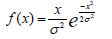
Normal distribution: The Normal distribution is widely used due to its simplicity and the central limit theorem, which assures that the distribution of sample means approximates a normal distribution as the sample size becomes large. However, it is less frequently used directly for lifetime data due to its support on the entire real line rather than just positive times.

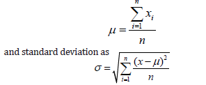
Density function is given with the formula and

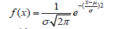
cumulative function with

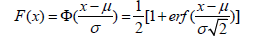
Where the parameters are:
μ-mean value
σ-standard distribution

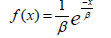
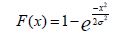
Exponential distribution: The exponential distribution is a continuous probability distribution that is frequently employed in reliability engineering and life data analysis. It is characterized by its simplicity and memoryless property, which makes it a preferred choice for modeling the time between events in a Poisson process.

The distribution is defined by a single parameter, the rate parameter, β, which is the reciprocal of the mean. This makes it particularly useful for scenarios where the event rate is constant over time, such as the time between arrivals of customers in a queue or the lifespan of electronic components.

Density function is given with the formula:

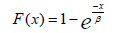
and cumulative function with:

Rayleigh distribution: The Rayleigh distribution can model failure times that result from the magnitude of a vector composed of random Gaussian components. It is often applied in scenarios where stresses have a random, directional nature.

Density function is given with the formula:

and cumulative function with:

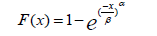
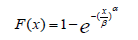
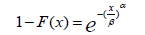
Weibull distribution: The Weibull distribution is one of the most versatile tools in reliability engineering. It can represent decreasing, constant, or increasing failure rates and is thus popular for modeling a wide range of failure modes [4,5].

Density function is given with the formula:

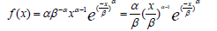
and cumulative function with:

Parameter estimation methods

The accuracy of parameter estimates is important for the reliability analysis. There are several methods to estimate these parameters, including Maximum Likelihood Estimation (MLE), the Method of Moments, and Ordinary Least Squares (OLS) regression. Each technique has its strengths and is chosen based on the nature of the data and the required precision of the estimates. Maximum Likelihood Estimation (MLE) is renowned for its desirable statistical properties, such as consistency, efficiency, and asymptotic normality. It involves finding the parameter values that maximize the likelihood function, thereby making the observed data most probable. The Method of Moments, on the other hand, is simpler and involves equating sample moments to population moments to solve for parameter estimates. Ordinary Least Squares (OLS) regression is particularly useful for linear relationships and involves minimizing the sum of the squared differences between observed and predicted values [5]

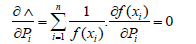
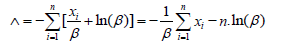
Maximum Likelihood Estimation (MLE): Maximum Likelihood Estimation (MLE) is a fundamental statistical method used for estimating the parameters of a probability distribution by maximizing the likelihood function, so the observed data is most probable under the assumed model. This method is particularly esteemed for its desirable statistical properties, such as consistency, efficiency, and asymptotic normality. The process begins with the formulation of a likelihood function, 𝐿, which expresses the probability of the observed dataset as a function of the parameters. Given that the product of probabilities can be computationally intensive, the natural logarithm of this function, known as the loglikelihood function (𝛬), is used. This transformation simplifies the multiplicative nature of the likelihood into an additive one, making the differentiation process more manageable. The next step involves deriving the partial derivatives of the log-likelihood function with respect to the parameters. Setting these derivatives to zero yields a system of equations, which, when solved, provide the MLE estimates of the parameters [6]. The elegance of MLE lies in its ability to leverage all available data, thus producing parameter estimates that are statistically optimal under large sample conditions. However, it is worth noting that MLE can be computationally intensive and may require sophisticated numerical methods for solving the resulting equations, particularly for complex models. The method is based on the maximization of the Probability function, given by:

That is, since the logarithm of the product is equal to the sum of the logarithms, the function is introduced:

Then the partial differentials are derived from the parameters and a system of equations is obtained:

The method of moments: The Method of Moments for parameter estimation involves equating sample moments-such as the sample mean and sample variance-to their corresponding population moments, thereby yielding equations that can be solved for parameter estimates. This technique is grounded in the principle that the moments of a sample should approximate the moments of the underlying population from which the sample is drawn. By setting the sample moments equal to the theoretical moments, one can derive estimators for the population parameters. Although simpler and computationally less demanding than Maximum Likelihood Estimation, the Method of Moments can be less efficient, particularly for small sample sizes, and may not always yield unbiased estimates. Nonetheless, it is a valuable tool in statistical inference, especially when dealing with simpler models or when computational resources are limited [7].

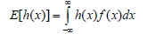
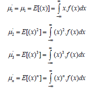
The expectation per function h(x) of a random variable x is denoted by E(h(x)) and is defined by:

The moment of the order r (r=1, 2, 3, ...) around the point b is defined as:

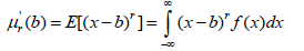
When b=0, then the moment is simply called the r^th the random variable x around the starting point 0 and is denoted by μ'_r.When b=E(x), then the moment is called the rth central moment of the random variable x and is denoted by μ._r The central moments are defined as: moment of

The moments around the starting point are defined as:

If there exists a moment of order n, then there are also moments of order k, where k< n.

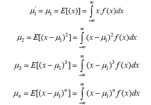
a) Central moments

i. The mean of the random variable x is equal to μ.₁ It is dependent on the shift.
ii. μ₂ =σ² = var(x) , This is called the variance of the random variable x, which is the square of the standard deviation of the random variable x. It doesn’t depend on shifting.
iii. Skewness is defined as:

iv. Kurtosis is defined as:

v. A mode value is defined as the value of a random variable with the highest frequency. In the case of a continuous distribution function in which there are first and second derivatives, mode, or m0 is the solution of the equations:

b) Some formulas

i.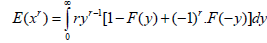 is the cumulative distribution function.
ii.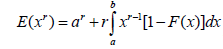 where a is a finite value and b is a finite or infinite value.
iii. The relationship between the central moments and the moments about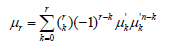
iv. That is, for the first 4 moments: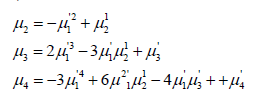

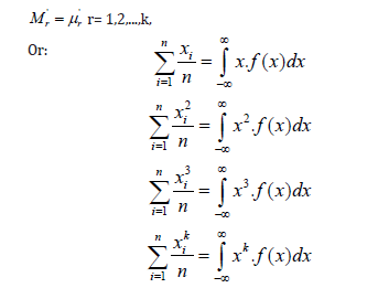
c) Determining the parameters of the distribution using moments

The R^th moment of the population is defined as:

If there are existing sufficient number of moments r'_μ as there are parameters to be evaluated, then a system of equations can be derived from the equation:

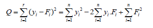
Linear regression: Linear regression is a fundamental statistical method used for modeling the relationship between a dependent variable and one or more independent variables. The essence of the method lies in fitting a line through a set of data points in such a way that the sum of the squared differences between the observed values and the values predicted by the line is minimized. This line, known as the regression line, is determined by estimating the parameters of the linear equation, typically using the least squares method. By doing so, linear regression provides a way to predict the dependent variable based on the values of the independent variables, making it a powerful tool for understanding and predicting trends and relationships in data. The basis of the method is to determine the parameters of the distribution (function) so that the square of the distance of statistically obtained values (points) and a given distribution function is minimal. Thus, the basic formula for the square of the distance is given by:

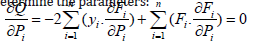
The minimum function of the square of the distance is obtained as zero of the partial derivatives of the function by each of the parameters to be determined, which gives a system of equations sufficient to determine the parameters:

Practical parameter estimation

In the following paragraphs we derive the formulas for the practical parameter estimation based on one or more methods described above. By applying the principles of linear regression, maximum likelihood estimation (MLE), or the method of moments, we can systematically obtain the parameters that best describe our data.

Normal distribution: Normal distribution parameters are straightforward to calculate, since they present the basic sample statistics.

Mean value is directly calculated from the function

This form allows for simple manual or spreadsheet calculation.

Exponential distribution: The simplest method for parameter estimation for this type of distribution is based on the MLE method.

Beta calculation in the basic formula substitution

From this form, one calculates the partial derivative by the parameter β and set it to zero.

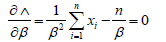
That is, if we reject a trivial solution that does not satisfy the initial conditions (b = 0), we obtain that:

This formula is trivial for the implementation in any spreadsheet program or manually calculated.

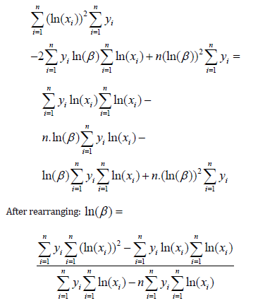
Weibull distribution: The most suitable form for direct implementation and manual/spreadsheet calculation can be achieved by implementing the linear regression.

The equation can be rewritten in the form:

Finally, the equation is transformed and the substitution is made

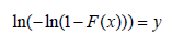
Which is the form that is simple to implement for linear regression:

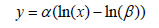
The partial derivatives of the function by parameters are given by the following:

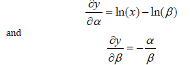
The partial derivative of the parameter a substitution is then applied in the form of the equation for the linear regression:

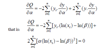
That is, after rearrangement, it is obtained that:

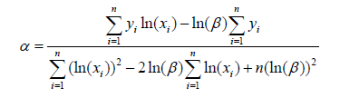
The partial derivative of the parameter b substitutions is then applied in the form of the equation for the linear regression:

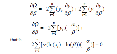
After rearranging:

If we set those two equations are equal, we get that:

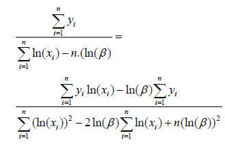
That is, after multiplying both sides:

Once the parameter β has been calculated, it is substituted back in the above equation and parameter α is calculated. Note on the values of y_i–that is, the values calculated based on the cumulative probability of failures – in the simplest form, they can be obtained in the following form – sort the data ascending based on the values x_i, and then calculate the F_i(x_i)=i/n, where n is the total number of points in the sample.

Rayleigh distribution: Rayleigh distribution is, by its basic formula, very similar to the exponential distribution. The easiest form for the direct parameter estimation can be obtained using MLE approach.

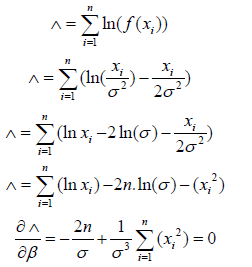
Solving by σ, the value is then calculated as

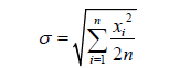
This form is convenient for direct estimation of the parameters.

Practical implementation

In order to demonstrate the practical application of the developed formulas, we consider a dataset consisting of 60 tensile tests conducted at room temperature for the material 10CrMoVNb9-1 (N168). The primary focus is on estimating the parameters of the distribution and assessing the goodness of fit using the square deviation method. For this purpose, we have compiled the experimental data in a comprehensive table format. This table includes the necessary columns for calculating the individual sums required by the previously derived formulas. The parameter estimation is carried out directly by implementing the formulas in Microsoft Excel. This method proves to be both efficient and accurate, ensuring that the parameters are estimated with a high degree of precision. The Excel implementation allows us to easily handle the computational requirements and verify the results through automated processes. By using Excel, we can take advantage of its built-in functions and tools, such as the goalseek function, which aids in optimizing parameter values for the best fit. Upon analyzing the data, we observe an excellent fit to the normal distribution, indicating that the material properties follow a predictable pattern under the given testing conditions. Additionally, the Weibull distribution also shows a very good fit, further validating the reliability of the data and the robustness of the parameter estimation method. The further optimization of the alpha parameter for the Weibull distribution has been attempted through the minimization of the square deviation (Table 1). This optimization process involves iteratively adjusting the parameter until the deviation between the observed and expected values is minimized. The optimized value is very close to the initially obtained value with the derived formulas, demonstrating very good fit, but also the fact that the given approach might not always achieve the optimal solution. The fitting of parameters using exponential and Rayleigh distributions has shown a poor alignment with the given data. This is primarily because the data exhibits a characteristic failure pattern concentrated around specific values, rather than displaying a random failure distribution over time. Both the exponential and Rayleigh distributions are typically used to model random failure patterns, which is inconsistent with the observed data (Table 2).

Table 1:Experimental data and values used for.

Table 2:Implemented calculation of the cumulative probabilities and deviation assessment.

Statistical approaches to parameter estimation form the backbone of reliability engineering, enabling practitioner+s to translate time-to-failure data into actionable metrics. By selecting appropriate distributions and applying robust estimation techniques-whether linear regression on transformed data, MLE, or the method of moments-engineers can quantify product reliability and develop efficient maintenance strategies. Model validation and uncertainty quantification ensure that these predictions are wellfounded and beneficial for engineering decision-making. The paper shows simple implementation path for the parameter optimization that can be implemented straight-forward in any spreadsheet program or straight calculations. The focus is on a practical, engineering implementation of the methods that allow practical utilization in day-to-day work.

Our deepest gratitude goes to all colleagues working in the reliability and statistics fields. Your invaluable contributions and insights have significantly enriched this work.

The authors declare no financial or other conflicts of interest related to this work.

1. Lawless JF (2003) Statistical models and methods for lifetime data. Pp: 1-630.
2. Meeker WQ, Escobar LA (1998) Statistical methods for reliability data. Pp: 1-680.
3. Mann NR, Schafer RE, Singpurwalla ND (1974) Methods for statistical analysis of reliability and life data.
4. Abernethy RB (2004) The new weibull handbook.
5. Dodson B (2006) The weibull analysis handbook.
6. Nelson W (1990) Accelerated testing: Statistical models, test plans, and data analyses.
7. Relia Soft Corporation (2015) Reliability engineering resource website.