Some Properties of Periodic Systems of Difference Equations Which have Periodic Solutions

Difference equations are commonly used in mathematics, because they may be natural mathematical model to describe the discrete processes (eg., in combinatorics). In papers [1-5] difference equations are used as models of population dynamics, and in [6] difference equations are used for modeling in genetics. In [7] the dynamics of the ecological system is also described by the system of difference equations. Another area where difference equations have played a prominent role is numerical analysis. Here one would approximate a given differential equation, through a discretization method, by a difference equation. In [8], the authors adjust the difference schemes corresponding to the equations under study in order to guarantee agreement between differential and difference systems in the sense of stability of the zero solution. They obtain conditions under which perturbations do not violate the asymptotic stability of solutions to difference systems.

Many evolutionary processes are characterized by the fact that at certain moments of their development they undergo rapid changes. In the mathematical simulation of such processes, it is convenient to neglect the duration of this rapid change and to assume that the process changes its state by jumps. For instance, such changes by jumps are observed in mechanics (the action of clockwork and the change in the velocity of a rocket by the separation of a stage), in radio engineering (generation of impulses of various forms), in biology (the work of the heart and the growth of the cells), in control theory (impulse control and the work of an industrial robot), etc. Adequate mathematical models of such processes are the so-called systems with impulse effect. These systems are governed by both differential and difference equations. This also confirms the importance of studying qualitative properties of difference equations.

Consider the following system of difference equations

where n=0, 1, 2, . . . is the discrete time, x(n)=(x₁(n), . . . , x_k(n))ε^T R^k, (.)T is the sign of conjugation, X: Z+*R^k R is continuous in x. Denote by x(n) = x(n, n0, x0) the solution of system (1) coinciding with x0 = (X₀, , X₀, . . . , X₀)T under n=n₀. We also denote Z₊ the set of non-negative integers, N the set of positive integers, and Nn0 the set of nonnegative integers satisfying inequality n>n₀.

Definition 1

System (1) is called periodic with period qεN if X (n+q,x) X (n,x) ; moreover for r=1, 2, . . ., q 1 we have X (n+q,x) X (n,x) . Invariant sets of system (1) are very important in the study of difference equations. The simplest invariant sets of equations (1) are equilibrium positions and periodic solutions of systems of difference equations.

Definition 2

The point x∗ ∈ R^k is called an equilibrium position of system (1) if X (n, x*) = x∗ for all n∈Nn0.

Definition 3

The solution x(n) of system (1) is called periodic with period p∈N if

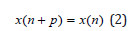
holds for all integers n Nn0. Geometrically property (2) means that the graph x(n) is repeated at all successive intervals of length p. Throughout this paper we assume that the period of solution x(n) is the smallest value p, satisfying (2). In this note we suppose that system of difference equations (1) is periodic with period q and this system has a periodic solution x(n) with period p. The purpose of this note is to clarify the possible relationship between p and q Elaydi & Sacker [9] proved the following theorem.

Theorem 1

Consider the periodic system of difference equations (1) with period q. If periodic solution M = x(n0), x(n1), . . ., x(np-1) of this system is globally asymptotically stable, then p is a divisor of q. In this theorem the authors showed the connection between the numbers p, q and the property of the periodic solution to be globally asymptotically stable. So, throughout this paper we shall consider the periodic system (1) with period q which has a periodic solution x(n) with period p without assumption of global asymptotic stability of this solution. Without loss of generality, we assume n0=0. We shall show that X(n, x) xεM is also periodic in n with period p. The following theorem is valid.

Theorem 2

If system of difference equations (1) has a periodic solution x(n) with period p, then function X(n, x) is also periodic with period p for xεM.

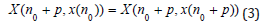
Proof: Let n0 0, 1, 2, . . ., p-1. Consider X(n0+p, x(n0)). The solution x(n) with initial point x(n0) is periodic with period p, hence,

According to (1) we find

On the other hand, from the periodicity of x(n) and (1) we have

From (3-5) it follows that X(n0, x(n0)) = X(n0+p, x(n0)), i.e. at all points of periodic trajectory M the relation X(n, x) = X(n+p, x) holds. This completes the proof.

Remark: Condition x εM is essential in Theorem 2 since without this condition this theorem is not true. As an example, consider the following system

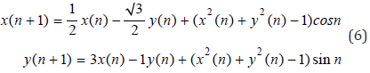
System (6) has the solution x(n) = cos πn/3, y(n) = sin πn/3 which is periodic with period p = 6, but right-hand sides of system (6) are periodic functions of n with period 2π. The chosen system has the property that the points of the plane x, y, through which solution x(n), y(n) passes (i.e. points of the unit circle x2+ y2=1) do not depend explicitly on the discrete time n. It turns out this is true not only for system (6), but also for any other system of difference equations (1) having a periodic solution whose period is incommensurable with the period of the system.

Theorem 3

Let system of difference equations (1) be such that X(n, x) is continuous function in n ε R, Xε Rk and periodic in n with irrational period q. If system (1) has the periodic solution M={x(0), x(1), . . . , x(p-1) with period pεN, then for any n0ε{0, 1, . . . , p-1} vectorfunction X(n, x(n0)) is constant. To prove this theorem, we need the following lemma which has been proven by Chebyshev [10] and its corollary.

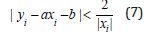
Lemma: If b is arbitrary real number, a is an irrational number, then there exist sequences of integer numbers { x_i}i^∞ = 1 and { y_i}i^∞ = 1 such that lim_i→∞ |x_i| =∞ ,lim_i→∞ |y_i| = ∞ and

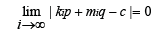
Corollary: Let p be an integer number, q-an irrational number. Then for any c∈R there exist sequences of integer numbers {ki}i^∞ = 1 and {mi}i^∞ = 1 such that limi → ∞ |ki| = ∞, limi → ∞ |mi| = ∞ and

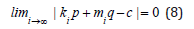
Proof of the corollary: It is clear that (8) is equivalent to the next limit relation

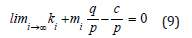
Since p is integer and q is irrational, q/p is also irrational. Letting q=a, yⁱ=kⁱ, xⁱ=mⁱ , c=b_pp, from inequality (7) we obtain

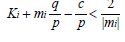
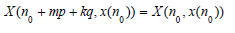
Bearing in mind that limi → ∞ |mi| = ∞ we get (9). The proof of the corollary is complete. Now let us prove. Theorem 3; Let m and k be arbitrary integer numbers. From periodicity of X and x we obtain

a

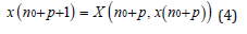
But according to (1) we have

x (n0+mp+1) = X (n0+mp, x(n0+mp)) (11)

On the other hand

x (n0+mp+1) = x (n0+1) = X (n0, x(n0)) (12)

From (10-12) it follows that for any integers m and k.

Let us show that

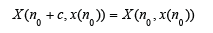
for any c ∈ R. Vector-function X is continuous, so all that we need is to show that there exist sequences of integer numbers {ki}i^∞ =1 and {mi}i^∞ = 1 such that , limi → ∞ |ki| = ∞ limi → ∞ |mi| = ∞

However, the existence of such sequences of integers

{ki}i^∞ = 1 and {mi}i^∞=1 follows from the above corollary. This completes the proof of Theorem 3.

1. Brauer F, Castillo CC (2001) Mathematical models in population biology and epidemiology. Springer, New York, USA.
2. Braverman E (2005) On a discrete model of population dynamics with impulsive harvesting or recruitment. Nonlinear Analysis 63(5-7): e751-e759.
3. Castro ML, Silva JAL, Justo DAR (2006) Stability in an age-structured metapopulation model. J Math Biol 52(2): 183-208.
4. Chen F (2006) Permanence and global attractivity of a discrete multispecies Lotka-Volterra competition predator-prey systems. Applied Mathematics and Computation 182(1): 3-12.
5. Franke JE, Yakubu AA (2006) Globally attracting attenuate versus resonant cycles in periodic compensatory leslie models. Mathematical Biosciences 204(1): 1-20.
6. Continho R, Fernandez B, Lima R, Meyroneinc A (2006) Discrete time piecewise affine models of genetic regulatory networks. J Math Biol 52(4): 524-570.
7. Jansen VAA, Lloyd AL (2000) Local stability analysis of spatially homogeneous solutions of multi-patch systems. J Math Biol 41(3): 232-252.
8. Yu Aleksandrov A, Zhabko AP (2003) On stability of solutions to one class of nonlinear difference systems. Siberian Mathematical Journal 44(6): 951-958.
9. Elaydi RS, Sacker J (2005) Global stability of periodic orbits of non-autonomous difference equations and population biology. Journal of Differential Equations 208(1): 258-273.
10. Chebyshev PL (1955) Selected works. Publisher of AS USSR, Moscow, Russia.