Autoencoder Based Multi-Class Classification Method For Alzheimer’s Disease Detection Using Brain MRI Data

Alzheimer’s Disease (AD) is an irreversible progressive neurological disorder characterized by progressive memory loss and a decline in activities of daily life, the retardation of thinking, and changes in personality and behaviors [1]. AD is the most common form of dementia that affects elderly people. AD causes nerve cells to die frequently, which leads to the loss of tissue in the brain that reduces the brain volume dramatically [2]. Mild Cognitive Impairment (MCI) causes serious cognitive changes that could be noticeable by the patient, in spite of that, the patient has the ability to perform everyday activities. People 60 years of age or older live with an MCI of 12-18%. In some individuals, MCI returns to a normal state or remains stable, on the other hand, the MCI could develop for various reasons, resulting in the MCI individuals going on to develop dementia. MCI can be at an early stage of AD if the hallmark changes in the brain are present [3]. A meta-analysis of 41 studies showed that the conversion rate from MCI to dementia when the individuals were tracked for 5 years or more, averaged at 38% [4]. It is for this reason that we focus on identifying patients with MCI so that clinicians can intervene timely and reduce the probability that a patient will progress to the Alzheimer’s Disease (AD) status.

In a recent paper on ADNI data classification, Ehsan Hosseini-Asl et al. [5] proposed to use a 3D convolutional neural network for feature extraction from MRIs. To be more specific, the authors of Ehsan HA et al. [5] used the Deeply Supervised Adaptive 3D-CNN (DSA-3D-CNN) which was initialized by training convolutional autoencoders for feature extraction and fine tuning the network for classification on different domain images. They showed impressive performance compared to the other approaches with binary ROC AUC over .96. This approach is the closest to the one we propose. An important note is that previous ADNI-based studies report results of a binary classification for the pairs of available classes, not a multiclass classification. In our study, we perform a multinomial classification and also test the performance of our proposed models so as to be able to compare our results with previous works. We have demonstrated that our approach achieves very good results without complicated preprocessing.

Our paper is the first paper that analyzes brain MRI scan images using Singaporean patients. In this paper, we demonstrate the end-to-end process from pre-processing (for example, brain skull stripping, cropping, resizing, intensity normalization, etc.) to classification of the patient as to whether they are Normal (NC), Mild Cognitive Impairment (MCI), Moderate Cognitive Impairment or have Alzheimer’s Disease (AD). We build two models for the classification of MCI using the EDNIS dataset that contains MRI brain scan images from Singaporeans. The first model uses a deep learning 3D Convolution Neural Network (3D-CNN) architecture (our baseline model), while our second model uses a generative network architecture, an Autoencoder (AE) model. The objective of our paper is to demonstrate that the Autoencoder performs much better in classifying MCI patients than a typical baseline 3D CNN model when analysing brain MRI scan images. We organize the succeeding sections as follows. Section 2 presents related work; Section 3 describes proposed network architecture. In Section 4, we present our experiments and results of our study. Finally, we conclude our findings in Section 5.

According to the latest report from Alzheimer’s Disease International [6], the number of people with dementia worldwide will increase from 50 million in 2019 to 152 million by 2050, and the global annual cost of dementia is estimated to increase from US $1 trillion in 2019 to US $2 trillion in 2030. Dementia is also the seventh-leading cause of death in the world [7]. Globally, dementia is a leading cause of death with a doubling in prevalence from 1990 to 2016 [8]. Due to the increasing burden of AD, methods for early detection and hence prevention of AD have become increasingly critical. CNNs first developed in the early 1990s [9]. However, due to restricted computational capabilities, they did not gain widespread appeal at the time. However, with the introduction of fast Graphics Processing Unit (GPU) computers and availability of labelled training data, CNNs have re-emerged as potent feature extraction and classification method, achieving record-breaking performance in a variety of significant computer vision issues. The success of CNNs in computer vision has motivated a large number of investigators in the medical imaging field, resulting in a flurry of publications in a short amount of time demonstrating the usefulness of CNNs for a range of medical imaging tasks [10]. Convolutional Neural Networks (CNNs) are deep multilayer artificial neural networks [11] that have the ability for quick feature extraction which makes them highly efficient in pattern recognition in image data analysis. They have been demonstrated to be highly accurate in image classification, in particular, medical imaging [12-14]. One of the advantages of CNNs over other neural network architectures is that it does not require manual extraction of relevant features based on prior knowledge. In image segmentation CNNs outperformed other algorithms, such as logistic regression and support vector machines that do not have intrinsic feature extraction capabilities [15]. CNN models, including several of the standard neural network algorithms, such as Google Net and Res Net have been proven effective at deep multi-classification analysis in medical imaging [12,16-19].

A special type of neural network, an autoencoder is a neural network that is trained by unsupervised learning, which is trained to learn reconstructions that are close to its original input. An autoencoder is composed of two parts, an encoder and a decoder. The difference between the original input vector x and the reconstruction output z is called the reconstruction error. An autoencoder learns to minimize this reconstruction error and uses the reconstruction error as the anomaly score. Data points with high reconstruction are considered to be anomalies. Only data with normal instances are used to train the autoencoder [20]. Baur C [21], provided the first application of deep convolutional representation learning for Unsupervised Anomaly Detection (UAD) in brain Magnetic Resonance (MR) images which operates on entire MR slices.

entire MR slices. A large amount of work in the field of deep learning based UAD has been devoted to Autoencoders (AEs) due to their ability to express non-linear transformations and the ability to detect anomalies directly from poor reconstructions of input data [22- 24]. Very recently, the first attempts have also been made with deep generative models such as Variational Autoencoders [20,25] (VAEs), however limited to dense neural networks and 1D data. Noteworthy, most of this work focused on the detection rather than the delineation of anomalies. Unfortunately, they suffer from memorization and tend to produce blurry images. Generative Adversarial Networks (GANs) [26] have shown to produce very sharp images due to adversarial training, however the training is very unstable and the generative process is prone to collapse to a few single samples. The recent formulation of VAEs has also shown that AEs can be turned into generative models which can mimic data distributions, and both concepts have also been combined into the VAEGAN [27], yielding a framework with the best of both worlds.

Anomaly GAN (Ano GAN) is a great concept for UAD in patch based and small resolution scenarios, but as experiments shown by Baur C [21] GANs lack the capability to reliably synthesize complex, high resolution brain MR images. Further, the approach requires a time-consuming iterative optimization. To overcome these issues [21] proposed the Anomaly Variational Autoencoder GAN (Ano VAEGAN) to build a model that captures “global” normal anatomical appearance rather than the variety of local patches. The reconstruction objective allowed them to train a generative model on complex, high resolution data such as brain MR slices. In order to avoid the memorization pitfalls of AEs and to improve realism of the reconstructed samples they trained the decoder part of the network with the help of an adversarial network, ultimately turning the model into a VAEGAN [20]. Baur C [21], in their experiments, compared the Ano VAEGAN against the Ano GAN framework and showed that the AE & VAE models with dense bottlenecks cannot reconstruct anomalies, but at the same time lack the capability to reconstruct important details in brain MR images such as brain convolutions. By utilizing spatial AEs with sufficient bottleneck resolution, i.e. 16X16 sized feature maps, they mitigated this problem. Noteworthy, a smaller bottleneck resolution of 8X8 size seemed to lead to a severe information loss and thus to large reconstruction errors in general. For future work, [21] intends to utilize 3D autoencoding models for unsupervised anomaly detection. This paper inspired us to classify Brain MRI Scan images using 3D autoencoder models for unsupervised anomaly detection.

Segmentation of Magnetic Resonance (MR) images is a fundamental step in many medical imaging-based applications. Traditionally, image segmentation is performed by having experienced clinicians scroll through a large number of 2D images and manually segmenting regions‐of‐interest among adjacent tissues. However, manual segmentation is time‐consuming and influenced by the level of human expertise and hence, there are errors associated with human interpretation. Manual segmentation is subject to inter‐ and intra-observer variability, which likely leads to inconsistent segmentation results [28]. There exist various segmentation methods like histogram-based thresholding, fusion algorithm and Expectation-Minimization (EM) based algorithm which gives promising results. These methods make use of the parametric and nonparametric approach to maximize the expectation level and these are not always suitable for all types of applications [29]. Otsu thresholding is a non-parametric approach for image segmentation and an alternative to Bayes decision rule [30].

Segmentation using Otsu thresholding gives the segmentation of image quickly with better segmentation accuracy results. (Add in our ROBEX info) The Liu F [31] study described a new fully automated CNN based segmentation method which integrated joint adversarial and segmentation CNNs to segment MR images with different tissue contrasts using a single set of annotated training data. This method was shown to provide rapid and accurate segmentation comparable to a state-of-the-art supervised CNN method. Additional studies are needed to evaluate potential applications of SUSAN for other anatomical structures and for other imaging modalities. The new technique may further improve the applicability and efficiency of CNN‐based segmentation of medical images while eliminating the need for large amounts of annotated training data (Figure 1).

Figure 1:Flow chart of this study.

Recently, deep neural networks have been applied successfully in image-to-image translation, particularly for improving image quality from one MRI modality to another [29]. A series of preprocessing steps were carried out. For example, skull stripping, bias field correction, pixel value normalization and data augmentation. The brain MRI structure is relatively complicated, and the cause of AD is not fully understood, most of the existing CNN-based methods are single scale representative features, and it is impossible to analyze the image information on the deep structure as most of the deformation of CNN is only stretched in the depth and width of the network structure, resulting in the model parameters that are too large to be used in practical applications. Pipelines used in a number of studies that applied deep learning algorithms to neuroimaging data mostly required multiple processing steps for feature extraction. Sergey Korolev [32] provided a powerful framework for automatic feature generation and more straightforward analysis. In this paper, Sergey Korolev [32] demonstrated how similar performance can be achieved skipping the feature extraction steps with the residual and plain 3D convolutional neural network architectures.

Following, Shmulev [33] and Senanayake [34] built 3D-ResNet and 3D-DenseNet, respectively, but their experimental results were not satisfactory. However, the small number of MRI data made the 3DCNN-based network difficult to fit completely. At the same time, the network had a larger number of parameters and longer training time. To address this issue, [35] proposed a novel Multi- Scale Convolutional Neural Network (MSCNet) to enhance the model’s feature representation ability for AD diagnosis. Compared with simple extraction of ROIs such as the hippocampus or sending raw AD data to CNNs for training, [35] first segment the MRI data into WM and GM. Then, a new and efficient network architecture with a multi-scale structure and channel attention mechanism was introduced to accurately classify images and to improve the interdependence between channels and adaptively recalibrate the channel direction’s characteristic response. Extensive experiments showed that [35] method achieved a good performance in AD diagnosis, and its model size was satisfactory. In addition, experiments proved that WM is more effective in the diagnosis of AD. But the data pre-processing and model training stages in [29] method was carried out separately.

The details of the process will be discussed in the following subsections.

Pre-processing of brain MRI images

Automatic whole-brain extraction from Magnetic Resonance Images (MRI), also known as skull stripping, is a key component in most neuroimage pipelines. As the first element in the chain, its robustness is critical for the overall performance of the system. Many skull stripping methods have been proposed, but the problem is not considered to be completely solved yet [36]. Many systems in literature have good performance on certain datasets (mostly the datasets they were trained/tuned on) but fail to produce satisfactory results when the acquisition conditions or study populations are different.

A robust, learning-based brain extraction system (ROBEX) method that combines a discriminative and a generative model to achieve the final result was introduced by [36]. The discriminative model was a Random Forest classifier trained to detect the brain boundary; the generative model was a point distribution model that ensures that the result is plausible. When a new image was presented to the system, the generative model was explored to find the contour with highest likelihood according to the discriminative model. Because the target shape was in general not perfectly represented by the generative model, the contour was refined using graph cuts to obtain the final segmentation. Brain segmentation, also known as skull stripping, is the problem of extracting the brain from a volumetric dataset, typically a T1-weighted MRI scan. This process of removing non-brain tissue is the first pre-processing step of most brain MRI image classification studies. Applications such as brain morphometry, brain volumetry, and cortical surface reconstructions require stripped MRI scans. Even early preprocessing steps such as bias field correction benefit from skull stripping. Automatic skull stripping is a practical alternative to manual delineation of the brain, which is extremely time consuming. Note that segmentation in MRI is in general a difficult problem due to the complex nature of the images (ill-defined boundaries, low contrast) and the lack of image intensity standardization [36].

In our study, we apply the automatic ROBEX software to do brain skull stripping. Figure 2 gives an example of ROBEX. It can give us a skull stripped image and a mask image for each input raw image. The skull stripped images are used for the next preprocessing steps. After getting the skull stripped images by ROBEX, we need to crop them by removing as many zero entries as possible without touching non-zero entries. We leave one voxel of zero padding around the obtained non-zero area in order to avoid sampling issues later on. The cropped images may have different sizes since they have different numbers of zero entries. Hence, we need to add paddings back to get the same size for all images. The last step is intensity normalization. We use Fuzzy C-means (FCM)- based tissue-based mean normalization in this study which is provided by intensity-normalization package [37].

Figure 2:An example of using ROBEX to obtain a skull stripped image and a brain mask image.

Training process

After the raw MRI are normalized using the process in Section 5.1, we will split the whole dataset into three parts: training dataset (70%), validation dataset (15%), and test dataset (15%). The validation dataset will be used for hyper parameter tuning and the details will be discussed in Section 5.4. The test dataset will be used for evaluating our models and the classification results are presented in Section 0. In this subsection, we use the training dataset to train the Autoencoder models (Figure 3).

Figure 3:Flowchart of pre-processing steps.

Autoencoder model

Autoencoder is an unsupervised artificial neural network which attempts to produce output identical to its input. The architecture of a typical Autoencoder has been introduced in Section 4. As mentioned before, when Autoencoder is used for anomaly detection, the threshold is always needed to detect whether the reconstruction error is large. However, deciding the threshold of reconstruction error is difficult and objective (Figure 4). Therefore, to overcome this difficulty, for the classification problem in this study, instead of training Autoencoder model on normal observations only, we trained k Autoencoder models for k classes separately. The training process of Autoencoder based multi-class classification method is described in (Figure 5).

Figure 4:An example of normalized MRI.

Figure 5:Training process.

We have three classes in this study, that is, NCI, CIND mild, and CIND moderate. We can train three Autoencoder models for the three classes based on NCI images, CIND mild images, and CIND moderate images from the training dataset, respectively. The three models are trained by minimizing the reconstruction errors between NCI images or CIND mild images or CIND moderate images and their reconstructed images, respectively. In this study, we use L₁-distance (Σⁿ₌₁image_i − reconstructed image_i where n is the size of the image, between the input image and reconstructed image as the reconstruction error.

Hyper-parameter tuning

We use Optuna tuner for hyper-parameter tuning in this study. Optuna [38] is an open-source hyper-parameter optimization framework to automate hyper-parameter search. To use Optuna tuner, we need to define an objective function, which is used to evaluate the performance of different trials. The tuner will run different sets of hyper-parameters and find the one that minimizes the objective function. In this study, we use the validation loss which is the L1-distance between the images in validation dataset and their reconstructed images as the objective function.

We usually use pruning or early stopping in deep learning so that we can develop a smaller and more efficient model. Optuna provides several pruners. We use the “Median Pruner” which applies the median stopping rule. Median stopping rule is a simple strategy, and it stops a trial if its performance falls below the median of other trials at similar points in time. To avoid the trail stops too early, we also add the “warmup _steps” option which means pruning is disabled until the trial exceeds the given number of steps.

To use the Optuna tuner, we need to specify the range of values of different hyper-parameters that we want to vary. Instead of randomly choosing a value from the given range, we decide to use “TPE Sampler”. This TPE Sampler applies Tree-structured Parzen Estimator approach [39], and it fits one Gaussian Mixture Model (GMM) l(x) to the set of parameter values associated with the best objective values, and another GMM g(x) to the remaining parameter values. It chooses the parameter value x that maximizes the ratio l(x)/g(x). However, we need to run at least 10 trials to let the TPE algorithm build the tree. If the number of trials is less than 10, random sampling is used.

Inference process

After the three models are trained based on the images from three classes, respectively, we can use them to classify new coming images. The inference process is described in (Figure 6). For a new coming image, we can get three construction errors by inputting it into the three Autoencoder models, respectively. This new observation will be assigned to the class with the smallest reconstruction error. The logic behind this lies in the fact that the autoencoders will be highly skilled at reproducing new data that is similar to data it has been trained on and vice versa. Therefore, the smallest reconstruction error given by the nth Autoencoder would imply that this new observation is closest in nature to the data corresponding to the nth class and as a result, we would assign this new observation to the nth class.

Figure 6:Inference process.

We ran a number of experiments to determine the number of layers, number of filters for each layer, learning rate, pooling size, batch size and dropout probability.

Dataset (based on 3 batches of images)

This study conducted the dataset from Epidemiology of Dementia in Singapore (EDIS) study. EDIS Study participants, aged 60-90 years, were drawn from the Singapore Epidemiology of Eye Disease (SEED) study, a population-based study among Chinese Singapore Chinese Eye Study [SCES], [40], Malays Singapore Malay Eye Study [SiMES-2],[41], and Indians Singapore Indian Eye Study [SINDI-2], [42]. These subjects can be divided into four classes based on the diagnosis of cognitive impairment and dementia, namely, No Cognition Impairment (NCI), Cognitive Impairment No Dementia (CIND) mild, CIND moderate, and Dementia. CIND was defined as impairment in at least one domain of NTB. The battery assesses seven domains which include five non-memory domains and two memory domains. CIND mild was diagnosed when ≤2 domains were impaired and CIND moderate as impairment of >2 domains. See more details at [40] and [43].

We have 537 T1 images in this EDIS dataset, among which 186 (30.44%) images are NCI, 156 (25.53%) images are CIND mild, 156 (25.53%) images are CIND moderate, and 39 (6.38%) images are dementia. Since the number of images in dementia is too small, we will only consider the classification problem for NCI, CIND mild, and CIND moderate classes in this paper. After the pre-processing, the normalized skull stripped images were resized to 174×174×174. 174 is decided by taking the largest number of non-zero entries for all images.

Implementation details (based on three batches of images)

We build upon the basic architecture of dense Autoencoder. All weights were initialized from a normal distribution with mean 0 and standard deviation 0.02. The encoder is a 3D convolutional neural network (CNN) that contains multiple layers. We set the number of channels in the input image for the first 3D convolutional layer as 1, and the number of channels produced by the first convolution as parameter “num_channels”. The number of layers in the encoder is determined by the parameters kernel_size (size of the convoluting kernel), stride (stride of the convolution) and num_channels. We limit the number of layers for encoder be less than 5 and set the kernel_size as (4,4,4), and stride as (2,2,2). The optimal values of stride and num_channels are selected by Optuna. The decoder is also a neural network that consists of multiple 3D de-convolutional layers. It performs a process that is opposite to that of the encoder. The encoder and decoder are connected by a fully connected neural network. The length of latent space z is the parameter called “embedding” which is also selected by Optuna. Moreover, we also use batch normalization [44] and ReLU [45] in both encoder and decoder and use dropout [46] with dropout rate 0.5 to avoid overfitting in the fully connected neural network. The architecture for the model trained on NCI data is presented in Figure 7 below.

Figure 7:The diagram of Autoencoder model trained by NCI images.

Hyperparameter tuning

All models were trained by using Adam optimizer with optimal learning rate selected by Optuna. The optimal parameters selected by Optuna for the three Autoencoder models are displayed in Table 1. Based on the optimal parameters selected by Optuna in Table 1, the structure of the Autoencoder model which was trained by NCI images is described in Figure 7. The structures of the Autoencoder models trained on CIND mild images and CIND moderate images are similar to that in Figure 7. Figure 8 above shows that the difference between the training and validation losses are minimal and close to 0. This shows that the three trained Autoencoder models were not overfitted and have reached convergence.

Figure 8:Loss plots of three Autoencoder models.

Table 1:Optimal parameters selected by Optuna for the three Autoencoder models.

Result

The unseen test dataset contained 57 images, which among 22 (38.59%) images are NCI, 15 (26.32%) images are CIND mild, and 20 (35.09%) images are CIND moderate. We used 4 measures to compare the performance of the methods we used, namely, overall accuracy, precision, recall, and f1-score. Except overall accuracy, the other three metrics are used for binary classification and the equations below indicates how to calculate them for each class:

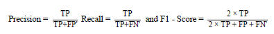
where FP, FN, TP, TN are given as false positives, false negatives, true positives, and true negatives, respectively. The classification results are presented in Table 2. The three autoencoders all performed well on the unseen brain MRI test images and managed to achieve an overall accuracy of 0.86. The F1 score and precision were also more than 0.7 for all three autoencoders.

Table 2:Classification results.

We proposed an autoencoder for the classification of brain MRI scans for MCI. We demonstrated performance of the convolutional neural networks and the autoencoder based on the EDNIS dataset which is a large available dataset of structural MRIs of Singaporean subjects with Alzheimer’s disease and normal controls. We showed that applying the proposed models to the MRI classification problem achieved results comparable to previously used approaches. The major advantage of our method is that there is no need for feature selection and the ease of use. Our proposed approach is useful for the automatic prediction of any given MRI scan for MCI. However, further studies will be needed to validate the autoencoder’s use in clinical practice.

A detailed examination and discussion on whether the SEED data is representative of the eventual target population and the possibility of sample biasness should also be conducted to support the generalizability of this study. For the eventual targeted deployment, issues such as model explanation and trustworthy computing will also be investigated, together with from-the-field insights. This will address any potential issues of biasness and showcase the robustness of the model. Further study in these directions is interested and warranted.

The authors declare that they have no known competing financial interests or personal relationships that could have appeared to influence the work reported in this paper.

1. Liu PP, Xie Y, Meng XY, Kang JS (2019) History and progress of hypotheses and clinical trials for Alzheimer’s disease. Signal Transduction and Targeted Therapy 4(1): 29.
2. Hosseini AE, Keynton R, El BA (2016) Alzheimer's disease diagnostics by adaptation of 3D convolutional network. 2016 IEEE International Conference on Image Processing (ICIP), Phoenix, Arizona, USA, pp. 126-130.
3. Alzheimer’s association (2021) Mild Cognitive Impairment (MCI) Alzheimer's Disease and Dementia.
4. Mitchell AJ, Shiri FM (2009) Rate of progression of mild cognitive impairment to dementia meta‐analysis of 41 robust inception cohort studies. Acta Psychiatrica Scandinavica 119(4): 252-265.
5. Ehsan HA, Georgy GF, Ayman E (2016) Alzheimer’s disease diagnostics by a deeply supervised adaptable 3D convolutional network. Arxiv.
6. World Alzheimer Report (2019) Attitudes to dementia. Alzheimer's Disease International, London, UK.
7. The top 10 causes of death. World Health Organization. (2020)
8. Nichols E, Szoeke CEI, Vollset SE, Abbasi N, Abd-Allah F, et al. (2019) Global, regional and national burden of Alzheimer’s disease and other dementias, 1990-2016: A systematic analysis for the global burden of disease study 2016. Lancet Neurology 18(1): 88-106.
9. LeCun Y, Boser B, Denker JS, Henderson D, Howard RE, et al. (1989) Backpropagation applied to handwritten zip code recognition. Neural Computation 1(4): 541-551.
10. Tajbakhsh N, Gotway MB, Liang J (2015) Computer aided pulmonary embolism detection using a novel vessel-aligned multi-planar image representation and convolutional neural networks. International Conference on Medical Image Computing and Computer-Assisted Intervention, Springer, Cham, Switzerland, pp. 62-69.
11. Albawi S, Mohammed TA, Zawi AIS (2017) Understanding of a convolutional neural network. International Conference on Engineering and Technology (ICET), Antalya, Turkey, pp. 1-6.
12. Liu Z, Luo P, Wang X, Tang X (2014) Deep learning face attributes in the wild. IEEE International Conference on Computer Vision (ICCV), Santiago, Chile, pp. 3730-3738.
13. Setio AAA, Ciompi F, Litjens G, Gerke P, Jacobs C, et al. (2016) Pulmonary nodule detection in CT images: False positive reduction using multi-view convolutional networks. IEEE Transactions on Medical Imaging 35(5): 1160-1169.
14. Wang SH, Phillips P, Sui Y, Liu B, Yang M, et al. (2018) Classification of Alzheimer’s disease based on eight-layer convolutional neural network with leaky rectified linear unit and max pooling. Journal of Medical Systems 42(5): 85.
15. Yan Z, Zhan Y, Peng Z, Liao S, Shinagawa Y, et al. (2016) Multi-Instance deep learning: discover discriminative local anatomies for bodypart recognition. IEEE Transactions on Medical Imaging 35(5): 1332-1343.
16. He K, Zhang X, Ren S, Sun J (2016) Deep residual learning for image recognition. IEEE Computer Society Conference on Computer Vision and Pattern Recognition (CVPR), Las Vegas, Nevada, USA
17. Szegedy C, Ioffe S, Vanhoucke V, Alemi AA (2017) Inception-v4, inception-ResNet and the impact of residual connections on learning. 31^st AAAI Conference on Artificial Intelligence, San Francisco, California, USA, pp. 4278-4284.
18. Khan S, Yong SP (2018) A deep learning architecture for classifying medical images of anatomy object. Asia-Pacific Signal and Information Processing Association Annual Summit and Conference (APSIPA ASC), Kuala Lumpur, Malaysia, pp. 661-1668.
19. Alsharman N, Jawarneh I (2020) Google Net CNN neural network towards chest CT-coronavirus medical image classification. Journal of Computer Science 16(5): 620-625.
20. Jinwon An, Sungzoon C (2015) Variational autoencoder based anomaly detection using reconstruction probability. SNU Data Mining Centre, 2015-2 Special Lecture on IE, pp. 1-18.
21. Christoph B, Benedikt W, Shadi A, Nassir N (2018) Deep autoencoding models for unsupervised anomaly segmentation in brain MR images. Computer Science, Springer, Cham, Switzerland.
22. Sabokrou M, Fathy M, Hoseini M (2016) Video anomaly detection and localization based on the sparsity and reconstruction error of auto-encoder. Electronics Letters 52(13): 1122-1124.
23. Hasan M, Choi J, Neumann J, Chowdhury AK, Davis LS (2016) Learning temporal regularity in video sequences. IEEE Conference on Computer Vision and Pattern Recognition (CVPR), Las Vegas, Nevada, USA, pp. 733-742.
24. Chong YS, Tay YH (2017) Abnormal event detection in videos using spatiotemporal autoencoder. Advances in Neural Networks, Springer, Cham, Switzerland, pp. 189-196.
25. Kingma DP, Welling M (2022) Auto-encoding variational bayes. ArXiv, pp. 1-14.
26. Goodfellow IJ, Pouget AJ, Mirza M, Xu B, Warde FD, et al. (2014) Generative adversarial nets. ArXiv, pp. 1-9.
27. Donahue J, Krähenbühl P, Darrell T (2016) Adversarial Feature Learning. ArXiv, pp. 1-18.
28. Ashton EA, Takahashi C, Berg MJ, Goodman A, Totterman S, et al. (2003) Accuracy and reproducibility of manual and semi-automated quantification of MS lesions by MRI. Journal of Magnetic Resonance Imaging 17(3): 300-308.
29. Tavares JMRS (2014) Analysis of biomedical images based on automated methods of image registration. Advances in Visual Computing, Springer, Cham, Switzerland, pp. 21-30.
30. Otsu N (1979) A threshold selection method from gray-level histograms. IEEE Transactions on Systems Man and Cybernetics 9(1): 62-66.
31. Liu F (2019) SUSAN: Segment unannotated image structure using adversarial network. Magnetic Resonance in Medicine 81(5): 3330-3345.
32. Sergey K, Safiullin A, Belyaev M, Dodonova Y (2017) Residual and plain convolutional neural networks for 3D brain MRI classification. 2017 IEEE 14th International Symposium on Biomedical Imaging (ISBI 2017), Melbourne, Victoria, Australia.
33. Shmulev Y, Belyae M (2018) Predicting conversion of mild cognitive impairments to alzheimer’s disease and exploring impact of neuroimaging. Graphs in Biomedical Image Analysis and Integrating Medical Imaging and Non-Imaging Modalities, Springer, Cham, Switzerland, pp. 83-91.
34. Senanayake U, Sowmya A, Dawes L (2018) Deep fusion pipeline for mild cognitive impairment diagnosis. 2018 IEEE 15th International Symposium on Biomedical Imaging (ISBI 2018), Washington, DC, USA, pp. 1394-1997.
35. Zhenbing L, Haoxiang L, Xipeng P, Mingchang X, Rushi L, et al. (2022) Diagnosis of Alzheimer’s disease via an attention-based multi-scale convolutional neural network. Knowledge Based Systems 238: 107942.
36. Juan EI, Cheng YL, Thompson P, Zhuowen T (2011) Robust brain extraction across datasets and comparison with publicly available methods. IEEE Transactions on Medical Imaging 30(9): 1617-1634.
37. Reinhold JC, Dewey BE, Carass A, Prince JL (2019) Evaluating the impact of intensity normalization on MR image synthesis. Medical Imaging 2019: Image Processing 10949: 890-898.
38. Akiba T, Sano S, Yanase T, Ohta T, Koyama M (2019) Optuna: A next generation hyperparameter optimization framework. 25th ACM SIGKDD International Conference On Knowledge Discovery & Data Mining, Anchorage, Alaska, USA, pp. 2623-2631.
39. Bergstra J, Bardenet R, Bengio Y, Kegl B (2011) Algorithms for hyper-parameter optimization. 24th Annual Conference On Neural Information Processing Systems (NIPS), Granada, Spain, pp. 2546-2554.
40. Hilal S, Ikram MK, Saini M, Tan CS, Catindig JA, et al. (2013) Prevalence of cognitive impairment in Chinese: Epidemiology of dementia in Singapore study. Journal of Neurology, Neurosurgery, Psychiatry 84(6): 686-692.
41. Hilal S, Tan CS, Xin X, Amin SM, Wong TY, et al. (2017) Prevalence of cognitive impairment and dementia in malays: Epidemiology of dementia in Singapore study. Current Alzheimer Research 14(6): 620-627.
42. Wong MYZ, Tan CS, Venkatasubramanian N, Chen C, Ikram MK, et al. (2019) Prevalence and risk factors for cognitive impairment and dementia in Indians: A multiethnic perspective from a Singaporean study. Journal of Alzheimer’s Disease 71(1): 341-351.
43. Yeo D, Gabriel C, Chen C, Lee S, Loenneker T, et al. (1997) Pilot validation of a customized neuropsychological battery in elderly Singaporeans. Neurological Journal of South East Asia 2: 123.
44. Ioffe S, Szegedy C (2015) Batch normalization: Accelerating deep network training by reducing internal covariate shift. 32nd International conference on machine learning, Lille, France 37: 448-456.
45. Nair V, Hinton GE (2010) Rectified linear units improve restricted boltzmann machines. 27th International Conference on Machine Learning, Haifa, Israel, pp. 807-814.
46. Srivastava N, Hinton G, Krizhevsky A, Sutskever I, Salakhutdinov R (2014) Dropout: A simple way to prevent neural networks from overfitting. The journal of Machine Learning Research 15(1): 1929-1958.