Modified Holt’s Linear Trend Method Based on Particle Swarm Optimization

Time series analysis and forecasting are very important for many scientific disciplines. In the literature, various forecasting methods were proposed. Exponential smoothing methods constitute a class of classical forecasting methods. According to component of time series, it is possible to use different exponential smoothing methods. First studies on exponential smoothing are Brown et al. [1-5] made a classification on exponential smoothing methods. Box et al. [6-9] studies tried to find equivalence among exponential smoothing methods and Autoregressive Integrated Moving Average (ARIMA) models. Hyndman et al. [10] obtain confidence intervals for forecasts of exponential smoothing methods. Yapar G et al. [11] studies proposed modified exponential smoothing methods by using time variant smoothing parameters. In this study, a modified Holt’s linear trend method is proposed. The proposed method uses second order update formulas apart from classical Holt’s linear trend model. In addition to modified update formulas, the proposed method us particle swarm optimization to estimate smoothing parameters and initial values of trend and level. In the second section Holt’s linear trend method is summarized. The brief information about Particle Swarm Optimization (PSO) is given in third section. In the fourth section the proposed method is introduced. The applications for real and simulated data sets are given in fifth section.

Holt [3] modified simple exponential smoothing for trend component. This method is called Holt’s linear trend method. In this method, level and trend of time series are estimated sample by sample in update formulas. Holt’s linear trend method uses following formulas:

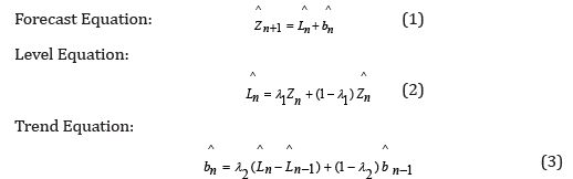
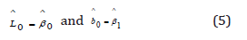
Right sides of (2) and (3) contain first order lagged terms. For calculating forecasts by using (1), initial values of level and trend is needed. Initial values can be obtained by estimating following regression equation.

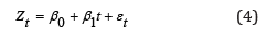
Least square estimations of β₀ and β₁ can be used as initial values of level and trend.

Indeed, Holt’s linear trend model is a kind of modification of (4) model. In (4) model level is fixed and trend is changing sample by sample using β₁t . In (4) model, trend value is increased as ^ β₁t amount. In Holt’s linear trend method, trend and level is changing sample by sample with equation (2) and (3). It is proved that forecasts of Holt’s linear trend method are equal forecasts of second order differenced and second order autoregressive model (ARIMA (0,2,2)).

Estimating statistical model parameters is very important task. Statistical methods required strong optimization methods for maximizing likelihood or minimizing sum of error squares. For linear models, there is no need iterative or strong optimization methods because the estimators can be obtained by solving linear equation systems. Derivate based iterative algorithms are used for non-linear statistical models. These algorithms trap local minima for many of statistical model applications. For some statistical models, derivate cannot be calculated at some points. Artificial intelligence optimization techniques do not need derivate of objective function and it can be remedy for nonlinear statistical model estimation. PSO is a stochastic and swarm optimization technique. PSO algorithm do not need derivate of objective function and it can avoid local optimum trap. PSO is firstly proposed by Kennedy and Eberhart (1995). The algorithm of modified PSO is given below:

Algorithm 1.

Step 1. Generate the initial positions and velocities from uniform distribution.

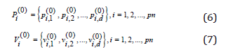
P_i(0) and V_i(0) present positions and velocities of ith particle, respectively.

Step 2. According to initial positions of each particle, fitness functions are calculated.

Step 3. Determine P_best and g_best

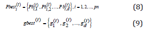
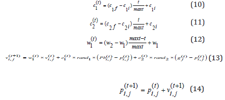
Step 4. Calculate new velocities and positions:

Step 5. Calculate the fitness function values for each particle.

Step 6. Update P_best and g_best . If the fitness value of g_best is smaller than pre-determined error tolerance, the training is ended for the bootstrap time series otherwise go to step 3,4.

Determining initial values of trend and level in Holt’s linear trend method is important problem and it effects forecasting accuracy. Estimating smoothing parameters is other important task in Holt’s linear trend method. A bound of Holt’s linear trend method is using first order update formulas. In this study, it is focused on these three issues. A modified Holt’s linear trend method is proposed [12]. The proposed method has new update equations for trend and level. Update equations of modified Holt’s linear trend method are given below:

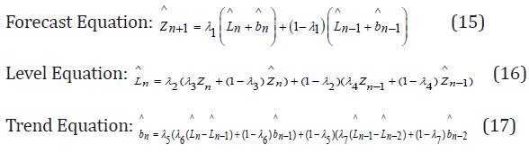
In the proposed method, λ_i ; i=01,2,..,7 smoothing parameters and is needed ^ L0 and ^ b0 initial values are estimated by using PSO method. Each particle has 9 positions and they are presented in Table 1.

Table 1: Positions of a particle in the proposed method.

Initial values for first two positions of a particle is generated from normal distribution. Firstly, (4) regression model is applied to time series and parameters are estimated in the model. After that initial positions of first two positions are generated from ^ N_{(β 0 , 0.01)} and ^ N_{(β 1, 0.01)} distributions. The initial positions of last seven positions are generated from uniform distribution with (0,1) parameters [13].

The performance of the proposed method is investigated by designing a simulation study. In simulation study, time series data sets are simulated by using following equations:

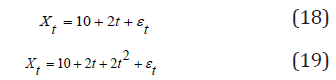
(18) is a linear trend, (19) is a quadratic trend model. The proposed method’s performance is compared with Holt’s linear trend method. In the generating series, the level of error variance is taken as 10, 100 and 1000. The length of test set is takes as 10, 20 and 30. For each situation 100 time series are simulated. After simulated series are analyzed by the proposed method and Holt’s linear trend method, minimum and mean statistics of RMSE values for test set are computed for each situation and listed in Table 2 & 3.

Table 2: Simulation results according to minimum of RMSE statistics.

Table 3: Simulation results according to mean RMSE statistics.

According to Table 2, the proposed method produced smaller RMSE value when the sigma level is 10. Moreover, the proposed method outperforms when the data generating process is quadratic trend model. According to Table 3 and mean statistics, the proposed method outperforms when the data generating process is quadratic trend model and smaller test set length. Secondly, Istanbul stock exchange data sets were analyzed by the proposed method, Autoregressive Integrated Moving Average Model (ARIMA), Multilayer Perceptron Artificial Neural Network (MLP-ANN) and Holt method. Istanbul stock exchange data sets is consisting of two time series which are daily observed in between 01.02.2009 and 29.05.2009 and between 01.04.2010 and 05.31.2010. The last 7 and 15 observations are used as test sets for both time series. The obtained results for test sets are given in Table 4-7. When the Table 4-7 are examined the proposed method is outperforms others for 2009 year. The proposed method is the second-best method for 2010 year and ntest=7. The proposed method is still the best method for 2010 year and ntest=15.

Table 4: The results of ntest=7 for Istanbul stock exchange data sets between 01.02.2009 and 29.05.2009.

Table 5: The results of ntest=15 for Istanbul stock exchange data sets between 01.02.2009 and 29.05.2009.

Table 6: The results of ntest=7 for Istanbul stock exchange data sets between 01.04.2010 and 05.31.2010.

Table 7: The results of ntest=15 for Istanbul stock exchange data sets between 01.04.2010 and 05.31.2010.

In this paper, a modified Holt’s linear trend method is proposed. The proposed method can determine initial values for trend and level. The proposed method uses second order update formulas, so it has better forecasting performance than classical Holt method. According to simulation study and real-world time series applications, the proposed method has smaller RMSE value for test sets than other alternative methods. In the future studies, the confidence intervals of the proposed method will be proved by using bootstrap techniques. Moreover, the similarity between ARIMA models and the proposed method will be examined.

1. Brown RG (1959) Statistical forecasting for inventory control. McGraw-Hill, New York, USA.
2. Brown RG (1963) Smoothing, forecasting, prediction. Englewood Cliffs, N.J.: Prentice-Hall, New Jersey, USA.
3. Holt CC (1957) Forecasting seasonal and trends by exponentially weighted moving averages. Office of Naval Research, Research Memorandum, 52.
4. Winters PR (1960) Forecasting sales by exponentially weighted moving averages. Management Science 6(3): 324-342.
5. Pegel CC (1969) Exponential forecasting: Some new variations. Management Science 15(5): 311-315.
6. Box GEP, Jenkins GM (1970) Time series analysis, forecasting and control. Holden Day, San Francisco, USA.
7. Roberts SA (1982) A general class of Holt-Winters type forecasting models. Management Science 28(7): 808-820.
8. Abraham B, Ledolter J (1983) Statistical methods for forecasting. John Wiley and Sons, New York, USA.
9. Abraham B, Ledolter J (1986) Forecast functions implied by autoregressive integrated moving average models and other related forecast procedures. International Statistical Review 54(1): 51-66.
10. Hyndman RJ, Koehler AB, Ord JK, Snyder RD (2005) Prediction intervals for exponential smoothing state space models. Journal of Forecasting 24: 17-37.
11. Yapar G, Sedat C, Hanife TS, Idil Y (2017) Modified Holt's linear trend method. Hacettepe Journal of Mathematics and Statistics, pp. 1394-1403.
12. Gooijer JGD, Hyndman R (2006) 25 Years of time series forecasting. International Journal of Forecasting 22(3): 443-473.
13. Johnston FR, Harrison PJ (2017) The variance of lead-time demand. Journal of Operational Research Society 37(3): 303-308.

© 2020 Egrioglu E. This is an open access article distributed under the terms of the Creative Commons Attribution License , which permits unrestricted use, distribution, and build upon your work non-commercially.