Decoding Brain’s Electrical Activity: Leveraging Hilbert Transforming Techniques for EEG Analysis

Analysis of raw EEG data remains a complex problem. EEG is a vast and complicated provider of multiple information and, at the same time, is vulnerable to noise and artifacts [1]. Thus, understanding what can be inferred from this delicate dynamic dance of electrical activity requires modern analytics. EEG and other electrophysiological recordings may help elucidate the complex computations in the brain [2]. The Fourier Transform is the groundwork of EEG analysis [3]. A traditional measurement tool for analyzing any waveform breaks it down into parts by their frequency content [4]. This breakage enables peak frequencies associated with a state of the brain. Some examples are slow waves associated with deep sleep, alpha waves linked with relaxation and beta waves aligned with focused attention [5]. By understanding which frequency bands are activated within the EEG spectrum, researchers can use them to access the underlying brain activity quickly. Short-Time Fourier Transform (STFT) takes the analysis to the next level [6]. The STFT assumes that the signals are dynamic but not steady and, hence, represent them in the time-frequency domain [7]. Also, there is another technique, called spectrogram, which is representing color intensity by the strength of each frequency while remaining consistent over time [8]. When applying it to EEG, this allows us to see sections of the brain “activate” and “inactivate,” which reveals how brain activity as represented by EEG bands alternates as one ponders or receives a stimulus of any kind [9,10]. The underlying signal of raw EEG data is distorted by noise and artifacts. That is when Contrast Limited Adaptive Histogram Equalization (CLAHE) comes into play [11]. CLAHE is a pre-processing technique that works by increasing the contrast of the low-contrast regions to better show their details [12]. It is like changing the contrast and brightness of an image to enhance hidden features. CLAHE enables increased signal quality of raw EEG data, allowing later transformers to perform more precise and robust analysis.

The understanding of the phase relationships between various brain regions is critical for the processing [13] such as the aspect of the EEG signal measured using the Hilbert Transform. An imaginary component of an actual signal is developed, which can then be used to establish the analytical signal. Based on this imaginary signal, it becomes possible to extract the instantaneous phase information of the EEG signal, which is pivotal in describing the rapidly changing brain connectivity and oscillatory patterns. Consider the analysis of the timing relationship between electrical activity of different brain areas as they correlate to perform cognitive functions [14]. Proper interpreting EEG provides possibility for innovative methods in the analysis of complex neural data, such as Machine Learning [15]. In this study, we are interested in applying Hilbert Transformation to the EEG data to enrich the ML models’ feature input, thus improve the performance of brain signal classification and analysis. The basis of comparison for all our metrics was the FFNN model, whether we feed the original signal or the Hilbert Transform data. The data was preprocessed, and after normalization, both the original EEG signal and the HL-applied EEG signal were fed into the FFNN model with the test accuracy used to compare the effects of HL on the original features. Our objective was to examine Hilbert Transformation impact, which gives a broader analytical view of the signal Amplitude envelope and the instantaneous phase, contributes to enriching the input Features better. Therefore, the other metric that we used to compare the impact of STFT, spectrograms, and CLAHE on the analysis of EEG data was CNN. The STFT, spectrogram, and CLAHE respectively applied to the zero-centered signal data processor, and to compare the test accuracies achieved by the CNN model. These metrics; FFNNs, and CNNs, enable us to exhaustively compare the signal processing techniques and choose the most effective in improving ML model performance for the classification of EEG signals. In addition, it should be considered that FFNN and CNN are the most primitive forms of neural networks. Due to their high sensitivity to input data, these models have been used as benchmark models in this paper; if the data is correctly pre-processed, it would boost the quality of the data prepared for the input of the neural network. Furthermore, it is critical to note that in the considered study the input data are kept constant by not performing the data shuffling procedure at any time during the study. Additionally, all hyperparameters for the two model types, FFNN and CNN, were frozen. Therefore, any increase in test accuracy could be exclusively attributed to the type of pre-processing technique conducted to the input data.

Dataset description

In this work, the SEED-V dataset [16] was employed, which is an advanced multimodal dataset created by the BCMI laboratory. The dataset is a cornerstone of many tasks in emotion recognition by providing both EEG signals as well as eye movement attributes in five emotional conditions: happiness, sadness, fear, disgust, and neutrality. More specifically, we mainly considered the emotional EEG data inside SEED-V; this allowed us to use this standardized data source to evaluate our methods. With over 5,800 applications performed by more than 1,000 research organizations up to December 2023, the SEED series datasets demonstrate remarkable significance and prospects for use in academia.

Evaluation methodology

Our methodology employed FFNNs and CNNs to evaluate test accuracy as metrics for our models. Our primary focus lies on the emotional EEG data, which we utilize to evaluate our analytical models. FFNNs are used for the Hilbert-transformed and original EEG signals, and CNNs are used to assess the efficacy of other image-based signal processing techniques such as STFT, spectrograms, and SCLAHE. Initially, we normalized data and froze all hyperparameters. This approach allowed us to maintain a consistent input format, avoiding data shuffling to ensure repeatable and reliable results. For the Hilbert Transformer evaluation, the normalized EEG signals were first classified using an FFNN. We measured the test accuracy to establish a baseline for EEG data classification. Subsequently, we applied the Hilbert Transformer to the EEG data and repeated the classification process, comparing the test accuracies to evaluate the impact of this preprocessing step. This iterative approach, with fixed hyperparameters for both the FFNN and CNN models, ensured that any observed improvements in test accuracy could be attributed to the enhanced quality of input data provided to the neural networks. Furthermore, we conducted comparative analyses using STFT, Spectrogram, and SCLAHE preprocessing techniques, employing a consistent CNN architecture as a classifier. These comparisons aimed to determine the efficacy of different preprocessing methods in improving model accuracy by introducing additional features into the input data. It is important to note that while EEG datasets are inherently time series sequences, typically suggesting a preference for other types of neural network architectures, our methodology justified the use of FFNNs and CNNs. By augmenting the EEG data with extra features through preprocessing, we hypothesized that if the preprocessing was effective, it would be reflected in increased test accuracy of the models. This approach is designed to demonstrate that, despite the conventional wisdom regarding neural network applications to time series data, significant improvements can be achieved through strategic data preprocessing.

Fourier transform

Brain signals’ complexity and variability, coupled with noise and artifacts, often render raw EEG traces challenging to interpret directly [17]. This complexity limits our ability to distinguish brain activities associated with different tasks or states directly from raw EEG signals. One of the pivotal mathematical tools used to overcome these limitations is the FT. The invention of the Fast Fourier Transform (FFT) by Cooley and Tukey in 1965 revolutionized signal processing, enabling efficient frequency analysis of EEG data [18]. This led to the broader adoption of the FT for EEG analysis. The FT is a mathematical transform that decomposes a function (often a time-domain signal) into its constituent frequencies [19]. For a continuous, time-domain signal x(t), the Fourier Transform X(f) is given by:

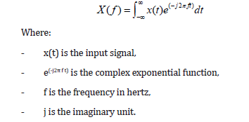
By decomposing a signal into its constituent frequencies, the FT enables researchers to analyze the spectral content of EEG data, providing insights into the brain’s rhythmic activity that is not readily apparent in the time-domain waveforms [20]. Applying the FT to EEG data facilitates several advantages over analyzing raw EEG signals [21]. Many noise sources and artifacts in EEG data, such as power line interference or muscle activity, have characteristic frequencies [22]. By analyzing the frequency spectrum of EEG data, researchers can more easily identify and filter out these unwanted signals, improving the signal-to-noise ratio and the reliability of the data. Changes in specific bands of the EEG frequency spectrum are associated with different cognitive and motor tasks. By examining changes in the power spectral density within these bands, we can distinguish between brain states associated with various tasks, even when such differences are not discernible in the raw EEG waveforms. Although the FT itself does not directly provide temporal information about when specific frequencies occur, extensions of the FT, such as the STFT and wavelet transforms, allow for the analysis of how the frequency content of EEG signals changes over time [23]. This capability is vital for studying dynamic brain processes.

Short-time fourier transform

The STFT addresses a crucial limitation of the basic FT when applied to EEG data, which is the lack of temporal resolution in the frequency domain [24]. While the FT is adept at revealing a signal’s frequency components, it does not provide information about when these components occur in time [25]. This limitation is particularly problematic for EEG analysis, given the brain’s dynamic nature, where the significance of neural oscillations can vary dramatically over short periods. The STFT is used to determine the sinusoidal frequency and phase content of local sections of a signal as it changes over time [26]. The STFT of a signal is obtained by multiplying the signal by a window function that slides over time:

Where:
- w(t-τ) is the window function centered around τ,
- f is the frequency,
- τ represents the time around which the window function is centered.

The STFT extends the FT’s capabilities by dividing the EEG signal into short, overlapping time segments and applying the Fourier Transform to each segment individually. This process results in a two-dimensional signal representation, where one axis represents time and the other frequency. In this work, we implemented STFT to analyze the non-stationary nature of EEG signals over time. Time-frequency representations Spectrograms were created, illustrating the evolution of frequency bands over cognitive tasks or stimuli. Thus, the STFT provides a time-varying frequency spectrum of the EEG signal, offering insights into how the power of different frequency bands evolves over an experiment or cognitive task. The STFT facilitates examining transient brain activities and their evolution over time [27]. By providing a timefrequency representation of EEG data, the STFT allows us to pinpoint the frequency components present in the signal and when these components occur [28].

This dual information is critical for understanding brain dynamics during different cognitive processes or in response to external stimuli. Similar to the FT, the STFT identifies artifacts with distinct time-frequency signatures. However, its time-resolved nature allows for more precise artifact removal. It can identify when the artifact occurs, enabling targeted filtering that preserves the integrity of the underlying brain signal. However, the choice of duration of each time segment requires a trade-off between time and frequency resolution; a larger window provides better frequency resolution but worse time resolution, and vice versa. This trade-off is known as the Heisenberg uncertainty principle of signal processing. Despite this limitation, the STFT’s ability to provide a time-resolved frequency analysis makes it an invaluable tool in EEG research. It allows a more nuanced understanding of brain activity’s complex, dynamic patterns, facilitating advances in neuroscience, clinical diagnostics, and brain-computer interfaces.

Spectrogram

A spectrogram is a visual representation of a signal’s spectrum of frequencies as it varies with time. The spectrogram is the squared magnitude of the STFT and is represented as:

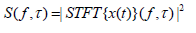
The spectrogram provides a 2D representation of the signal [29]. One axis represents time, the other frequency, and the intensity of each point represents the magnitude of the frequency at that time. In EEG analysis, the spectrogram plays a crucial role by offering a compelling and intuitive way to examine and interpret the complex dynamics of brain electrical activity [30]. Creating a spectrogram involves dividing the EEG signal into short, overlapping segments, applying the Fourier Transform to each segment to obtain its frequency spectrum, and then plotting these spectra as a function of time [31]. The result is a two-dimensional graph with time on the horizontal axis and frequency on the vertical axis. The intensity of each frequency at each point in time is represented by the color or brightness of each point on the graph. This transformation enhances the detection of specific brain activities that might be less apparent in standard spectral analyses. The Transformed of Spectrum analysis leverages advanced signal processing techniques to isolate and magnify features within the EEG data, offering a new layer of insight into the neural dynamics underlying different cognitive states and responses to stimuli [32]. Spectrograms provide a clear, visual means of identifying changes in brain activity over time. This includes the onset and offset of specific frequency bands associated with different cognitive states or responses to stimuli, offering immediate insights that might be less apparent through numerical analysis alone. Spectrograms maintain the inherent trade-off between time and frequency resolution due to the Heisenberg uncertainty principle. However, they allow researchers to visually assess the balance between these resolutions and adjust their analysis parameters accordingly (Table 1).

Table 1:Improvement of neural network accuracy by applying transformations on EEG data.

Contrast limited adaptive histogram equalization

Applying CLAHE to EEG signal analysis represents an innovative crossover from image to biomedical signal processing. Traditionally, CLAHE is utilized to enhance the contrast in images, particularly in contexts where it’s crucial to identify details obscured by poor lighting or similar factors [33]. Its adaptation for EEG signal analysis involves an abstract yet insightful approach, leveraging the technique’s core principles to enhance the interpretability of EEG data visualizations, such as time-frequency maps, brain topographies, and other graphical representations derived from EEG signals. The mathematical description of histogram equalization involves calculating the Cumulative Distribution Function (CDF) of the pixel intensities and mapping it to a new set of values to spread out the most frequent intensity values [34]. We break down the process into sequential steps to detail the CLAHE algorithm mathematically, especially considering an image as a matrix. Each step involves specific operations on the image’s pixel values. CLAHE is an image processing technique used to improve the contrast of images and unlike ordinary histogram equalization, CLAHE operates on small regions in the image, called tiles, rather than the entire image [35]. The algorithm enhances the contrast of each tile, so when the tiles are stitched back together, the contrast of the entire image is improved without significantly amplifying noise. The process is described as follows:

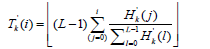
Divide the Image into tiles: Consider an image represented as a matrix I of size M×N, where M is the number of rows (height) and (N) is the number of columns (width). The image is divided into non-overlapping tiles of size (m×n). The number of tiles can be calculated as:

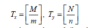
where T_x and T_y are the numbers of tiles along the x and y directions, respectively, and (⌈⋅⌉) denotes the ceiling function.

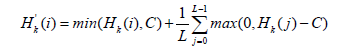
Apply histogram equalization to each tile: For each tile, we calculate its histogram H_k(i), where k is the tile index and i is the intensity level ranging from 0 to (L-1) (e.g., for an 8-bit image, (L=256). The histogram equalization transformation function T_k (i) for each tile is then given by:

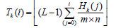
Clip the histogram (contrast limiting): To prevent excessive contrast enhancement, the histogram is clipped at a predefined threshold (C). If (H_k(i)>C), the excess is redistributed uniformly across all intensity levels. The clipped histogram ' (H_k)j is given by:

Calculate the new transformation function: Using the clipped histogram, we calculate a new transformation function 'T_k(i)for each tile:

Interpolation: To eliminate artificially induced boundaries between tiles, bilinear interpolation is applied using the transformation functions '( ) k T i of the four nearest tiles. For a pixel (x,y) within a tile, its new intensity I’ (x,y) is calculated as:

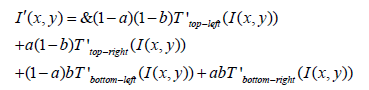
Where (a) and (b) are the horizontal and vertical distances of the pixel from the top-left corner of the tile it belongs to, normalized by the tile dimensions. This process enhances each region’s local contrast while controlling the image’s overall contrast enhancement to avoid amplifying noise. CLAHE is particularly effective for enhancing the contrast of medical images or photographs taken in low-light conditions. As CLAHE enhances contrast in localized regions within an image to reveal hidden details, applying it to EEG visualizations enhances the distinction between different signal components. This could improve the visibility of subtle oscillatory patterns, phase-amplitude coupling, or transient events like spikes and sharp waves, which are significant in diagnosing neurological conditions.

One of the critical challenges in EEG analysis is the presence of noise and artifacts, such as those caused by muscle movements, eye blinks, or external electrical sources [36]. The contrast-limiting aspect of CLAHE can be particularly beneficial in EEG visualizations by preventing the overamplification of noise, ensuring that genuine brain activity is highlighted without exaggerating the underlying noise and artifacts. While EEG signals fundamentally differ from photographic images, many forms of EEG analysis involve creating visual representations, such as spectrograms, topographic maps, or brain connectivity graphs [37]. Applying CLAHE to spectrograms or time-frequency plots of EEG data can make identifying specific frequency bands and their temporal dynamics easier, which is critical for understanding brain states and diagnosing disorders [38]. For EEG topographies that show the distribution of electrical activity across the scalp, CLAHE can enhance the contrast between regions of high and low activity, facilitating the localization of brain activity or abnormalities [39]. By limiting contrast enhancement in areas with minimal signal variability, which might otherwise amplify noise, CLAHE helps maintain a balance where the focus is on meaningful EEG signal components [40].

Hilbert transform

The Hilbert Transform is a fundamental tool in signal processing, particularly valued for its application in analyzing EEG signals [41]. This mathematical transform derives the analytic representation of a real-valued signal, enabling the extraction of its amplitude envelope and instantaneous phase [42]. Utilizing the Hilbert Transform in EEG signal analysis facilitates a deeper understanding of brain activity’s complex, oscillatory nature, offering insights into the amplitude and phase dynamics of neural oscillations across different brain states and conditions [43]. By applying the Hilbert Transform to EEG signals that have been filtered into specific frequency bands (e.g., delta, theta, alpha, beta, and gamma), researchers can isolate and analyze the dynamics of these bands [44]. This is particularly useful in studies related to sleep, cognition, and various neurological disorders, where different frequency bands are associated with distinct brain states and functions. The Hilbert Transform offers a robust framework for enhancing emotion classification tasks using EEG signals [45]. By providing a comprehensive time-frequency analysis, it enables the extraction of features that are crucial for distinguishing between different emotional states. The following subsections detail the application and benefits of the Hilbert Transform in this context.

Feature extraction: The Hilbert Transform facilitates extracting instantaneous features from EEG signals, such as amplitude, frequency, and phase. These features can directly correlate with various emotional states, offering a nuanced understanding of brain responses to emotional stimuli.

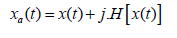
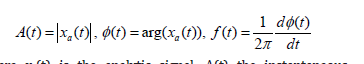
where x_a(t) is the analytic signal, A(t) the instantaneous amplitude, ϕ(t) the instantaneous phase and f(t) the instantaneous frequency.

Phase synchronization analysis: The phase information provided by the Hilbert Transform can be utilized to investigate the synchronization between different brain regions during emotional processing. This is crucial for understanding the network dynamics underlying different emotional states.

where Δϕ_ij(t) represents the phase difference between EEG signals from regions i and j.

Enhanced classification models: Features derived from the Hilbert Transform can significantly enhance the performance of machine learning models for emotion classification. By incorporating these features, classifiers can better distinguish between subtle differences in EEG signals corresponding to different emotions.

where the classifier uses instantaneous amplitude, frequency, and phase synchronization, among others, to predict the emotional state.

Temporal dynamics of emotions: The Hilbert Transform’s ability to capture the temporal dynamics of EEG signals allows for analyzing how emotional states evolve over time. This temporal aspect is critical to understanding the transient nature of emotions and their impact on brain activity.

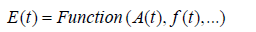
where E(t) represents an emotional state at time t, as a function of instantaneous amplitude, frequency, and other features.

In this investigation, a STFT was applied to two distinct emotional states, Happiness and Fear, extracted from the SEED-V dataset, as depicted in Figure 1. Upon analysis, it was observed that after the application of STFT, no intuitive or visually discernible differences between the ‘Happiness’ and ‘Fear’ categories could be identified. This lack of distinction suggests that when STFT is employed as a preprocessing technique, it introduces complexities for NN models in efficiently evaluating and classifying the processed data. It is intended to be empirically demonstrated within this study that this preliminary observation is accurate, thereby underscoring the challenges NN models encounter in classifying data that has undergone STFT preprocessing. Subsequently, an experiment was meticulously designed, wherein the data, processed through STFT from the SEED-V dataset, were input into a specifically configured Convolutional Neural Network (CNN) (Figure 2). The architecture of this CNN was meticulously crafted, incorporating two convolutional layers with filters set to a dimension of 3x3 and channel counts set at 32 and 64, respectively. Following the convolutional layers, a fully connected layer was introduced. This layer was designed with 128 neurons, employing the Rectified Linear Unit (ReLU) activation function, with the aim of classifying the Electroencephalogram (EEG) signals. This approach was chosen to meticulously address the classification challenges presented by EEG data that had been preprocessed with STFT, demonstrating the complexities and considerations involved in preparing EEG data for neural networkbased analysis. The utilization of STFT after integration into the CNN model yielded an accuracy of 22%. Figure 3. illustrates the training and validation losses. It is noteworthy to mention that CNN serves as the metric in our study, and it should be emphasized that achieving the maximum test accuracy for classification is not the primary objective.

Figure 1:Comparison of Happy (a and b) and Fear (c and d) conditions pre-STFT (a and c) and post-STFT (b and d) processing.

Figure 2:The CNN architecture used in this study.

Figure 3:The loss for training and validation after using STFT.

Based on the observations Figure 4, it was intuitively anticipated that the Happy and Fear classes would have more pronounced differences. Specifically, the image corresponding to the ‘Fear’ class exhibited a greater extent of red-colored areas, indicative of heightened distinctions between the two classes. Consequently, it was hypothesized that feeding spectrogram images to the CNN would yield higher accuracy compared to utilizing the STFT transformation alone. Indeed, the incorporation of spectrogram images into the CNN model resulted in an improved accuracy of 33%, surpassing the accuracy obtained with the STFT transformation, which stood at 22%. The training and validation losses are illustrated in Figure 5. In another method explored in this study, we initially applied Spectrogram transformation to the EEG signals. Subsequently, we subjected the data to CLAHE Transformation. As depicted in Figure 6, there are discernible differences between the CLAHE-Transformed data, indicating significant alterations in the data distribution. Consequently, it was anticipated that this preprocessing approach would lead to improved accuracy postclassification (Figure 7). Upon feeding these transformed data into the CNN model, a test accuracy of approximately 45% was obtained, surpassing the accuracies achieved with Spectrogram alone (22%) and Spectrogram followed by STFT (33%). This finding underscores the efficacy of combining Spectrogram and CLAHE transformations as a preprocessing step to enhance classification accuracy in EEG signal analysis. In Figure 8, it is evident that both the Happy and Fear classes display similar characteristics following the application of the Hilbert transformation. However, the true potency of mathematical techniques emerges through the Hilbert Transform’s ability to extract additional features.

Figure 4:Comparison of Happy (a and b) and Fear (c and d) conditions pre-Spectrogram (a and c) and post- Spectrogram (b and d) processing.

Figure 5:The loss for training and validation after applying Spectrogram Transformation.

Figure 6:Comparison of Happy (a and b) and Fear (c and d) conditions pre-SCLAHE (a and c) and post-SCLAHE (b and d) processing.

Figure 7:The loss for training and validation after using CLAHE Enhanced Spectrogram Transformation.

Figure 8:Comparison of Happy (a and b) and Fear (c and d) conditions pre-Hilbert Transformation (a and c) and post-Hilbert Transformation (b and d) processing.

Initially, when the raw EEG data was input into the FFNN network without undergoing any transformation, the accuracy plateaued at approximately 53%. This outcome implies that FFNN networks may not be optimally tailored for tasks involving time sequences. However, upon implementing the Hilbert transformation, a notable improvement in accuracy, reaching about 79%, was observed. Therefore, we conclude that applying the Hilbert transformation on raw EEG data could improve accuracy by 49%. Subsequently, both the original EEG data and the Hilberttransformed data were fed into the FFNN network. This network comprised four hidden layers, each housing 512 neurons with ReLU activation functions. It is pertinent to note that this neural network architecture is deliberately kept simple, and the study’s objective does not solely focus on maximizing accuracy. The schematic of the FFNN fully connected model is delineated in Figure 9. The loss curves for training and evaluation of both the original EEG data and the Hilbert-transformed data are depicted in Figure 10. By applying the Hilbert transformer to EEG data, we extract additional information for each EEG sample. These auxiliary features provide richer representations of the data, enabling the FFNN model to classify more accurately. Therefore, in the current EEG data analysis, the transformative techniques examined through this study are an essential aid in discovering the puzzle of the brain electrical signals. The FT is truly a bedrock for frequency analysis. Nevertheless, the method has its limitations on the treatment and resolution of non-stationary signals that call for methods that provide a timecore domain, such as the STFT. However, with its time-frequency representation, the method provides a limit in precision forfeiting the rapid neural dynamics subtleties. Preprocessing using the SCLAHE enhances the signal clarity, especially in discouraging noise, providing a clean ground for all the future process. The use of the Hilbert transformation and SCLAHE on preprocessing phase on our data inputs significantly reduce the computational complexity involved. This methodology is amazing due to its unique capabilities.

In problem areas where methods such as synchronization and brain connectivity flounder, the Hilbert Transform is almost the only thing that can be effectively applied. Given that the Hilbert methodology allows us to obtain the phase of the signal, which is fundamentally a more important area of research due to synchronization regions in the brain. Among the possible future work directions, one can note the integration of transformative technologies with advanced computational models such as deep learning. This integration will significantly increase the accuracy and granularity of EEG analysis, which will make it possible to open up completely new perspectives in the field of cognitive science and neurovascular engineering.

Figure 9:The schematic of FFNN fully connected classifier metric model.

Figure 10:The loss for training and evaluation for original EEG data (left hand-side) and Hilbert transformed data (right hand-side).

In this work, we investigated the effect of different preprocessing methods on the accuracy in EEG classification on the basis of SEED-V EEG dataset. Initially, STFT failed to show significant differences among states. But further checks with a CNN seemed to prove that using spectrogram images increased and produced more correct results than the STFT alone. Combining the Spectrogram and CLAHE transformations further enhanced accuracy, demonstrating the worth of multi-step preprocesses in this area. Moreover, our study of Hilbert transformations showed that they had a positive effect on the classification accuracy of raw EEG features. This suggests the importance of applying mathematical transformations to time sequence data for improved performance in processing. It was also pointed out that the accuracies of FFNN models with raw EEG data reach some limit. But factoring in the Hilbert transformation strikingly improved performance of the FFNN model with a notable 49% increase in accuracy, indicating ability to turn this transformation optimally delivering improvements in NN efficiency. In addition, by incorporating spectrogram images from STFT data the CNN architecture could be kept consistent with fixed hyperparameters throughout. Furthermore, the spectrogram data obtained a 50% accuracy improvement with this move. When CLAHE was applied to spectrogram data (SCLAHE), this improvement dramatically increased to a whopping 104%. This clearly highlights the combined strength of different pre-processing techniques on model accuracy in neural networks. Discussion the current research emphasizes the absolute importance of advanced preprocessing in EEG signal analysis. It proves that using transformations can have a large impact upon neural networkbased classification accuracy, and illuminates the fine details and necessary considerations involved in pre-processing raw EEG data for practical analysis.

This work received joint sponsorship from the National Science Foundation (NSF), under Award No. 1924278, and the National Institutes of Health (NIH), with Award No. IOT2OD032581-02 and Subaward No. 211014AS096-05.

1. Ranjan R, Sahana BC, Bhandari AK (2024) Deep learning models for diagnosis of schizophrenia using EEG signals: Emerging trends, challenges and prospects. Archives of Computational Methods in Engineering 10: 1-40.
2. Lotte F, Bougrain L, Cichocki A, Clerc M, Congedo M, et al. (2018) A review of classification algorithms for EEG-based brain-computer interfaces: A 10-year update. Journal of Neural Engineering 15(3): 031005.
3. Yamaguchi C (2003) Fourier and wavelet analyses of normal and Epileptic Electroencephalogram (EEG). In First International IEEE EMBS Conference on Neural Engineering, Capri, Italy.
4. Lyu F, Wang Y, Mei Y, Li F (2023) A high-frequency measurement method of downhole vibration signal based on compressed sensing technology and its application in drilling tool failure analysis. IEEE Access, USA.
5. Bellesi M, Riedner BA, Garcia Molina GN, Cirelli C, Tononi G (2014) Enhancement of sleep slow waves: Underlying mechanisms and practical consequences. Frontiers in Systems Neuroscience 8: 208.
6. Kizhakkel VR (2013) Pulsed radar target recognition based on micro-Doppler signatures using wavelet analysis. The Ohio State University, USA.
7. Akan, Cura OK (2021) Time-frequency signal processing: Today and future. Digital Signal Processing 119: 103216.
8. Dennis J, Tran HD, Li H (2010) Spectrogram image feature for sound event classification in mismatched conditions. IEEE Signal Processing Letters 18(2): 130-133.
9. Garrett DD, MacDonald SW, Lindenberger UA, McIntosh R, Grady CL (2013) Moment-to-moment brain signal variability: a next frontier in human brain mapping? Neuroscience & Biobehavioral Reviews 37(4): 610-624.
10. Çakar T, Filiz G (2023) Unraveling neural pathways of political engagement: Bridging neuromarketing and political science for understanding voter behavior and political leader perception. Frontiers in Human Neuroscience 17: 1293173.
11. Vutakuri N (2023) Detection of emotional and behavioral changes after traumatic brain injury: A comprehensive survey. Cognitive Computation and Systems 5(1): 42-63.
12. Sahu S, Singh AK, Ghrera S, Elhoseny M (2019) An approach for de-noising and contrast enhancement of retinal fundus image using CLAHE. Optics & Laser Technology 110: 87-98.
13. Sheng D, Pu W, Linli Z, Tian GL, Guo S, et al. (2023) Aberrant global and local dynamic properties in schizophrenia with instantaneous phase method based on Hilbert transform. Psychological Medicine 53(5): 2125-2135.
14. Almohammadi A, Wang YK (2024) Revealing brain connectivity: Graph embeddings for EEG representation learning and comparative analysis of structural and functional connectivity. Frontiers in Neuroscience 17: 1288433.
15. Saeidi M, Karwowski W, Farahani FV, Fiok K, Taiar R, et al. (2021) Neural decoding of EEG signals with machine learning: A systematic review. Brain Sciences 11(11): 1525.
16. https://bcmi.sjtu.edu.cn/home/seed/
17. Li Z, Zhang L, Zhang F, Gu R, Peng W, et al. (2020) Demystifying signal processing techniques to extract resting-state EEG features for psychologists. Brain Science Advances 6(3): 189-209.
18. Ojumah H, Atonuje A (2023) Cooley-Tukey type discrete fourier transform algorithm for continuous function sampled at some composite point N=pq, p≠ Nigerian Journal of Science and Environment 21(1).
19. Akan A, Cura OK (2021) Time-frequency signal processing: Today and future. Digital Signal Processing 119: 103216.
20. Zhou Y, Sheremet A, Qin Y, Kennedy J, DiCola N, et al. (2019) Methodological considerations on the use of different spectral decomposition algorithms to study hippocampal rhythms. Eneuro 6(4).
21. Sanei S, Chambers JA (2013) EEG signal processing. John Wiley & Sons, New Jersey, USA.
22. Mannan MMN, Kamran MA, Jeong MY (2018) Identification and removal of physiological artifacts from electroencephalogram signals: A review. IEEE Access 6: 30630-30652.
23. Arts LP, Broek ELVD (2022) The fast continuous wavelet transformation (fCWT) for real-time, high-quality, noise-resistant time-frequency analysis. Nature Computational Science 2(1): 47-58.
24. Gosala B, Kapgate PD, Jain P, Chaurasia RN, Gupta M (2023) Wavelet transforms for feature engineering in EEG data processing: An application on Schizophrenia. Biomedical Signal Processing and Control 85: 104811.
25. Boashash B (2015) Time-frequency signal analysis and processing: A comprehensive reference. Academic press, Massachusetts, USA.
26. Assous S, Boashash B (2012) Evaluation of the modified S-transform for time-frequency synchrony analysis and source localization. EURASIP Journal on Advances in Signal Processing 49 (1): 2012.
27. Gramfort A, Strohmeier D, Haueisen J, Hämäläinen MS, Kowalski M (2013) Time-frequency mixed-norm estimates: Sparse M/EEG imaging with non-stationary source activations. Neuroimage 70: 410-422.
28. Amiri M, Aghaeinia H, Amindavar HR (2023) Automatic epileptic seizure detection in EEG signals using sparse common spatial pattern and adaptive short-time Fourier transform-based synchro squeezing transform. Biomedical Signal Processing and Control 79: 104022.
29. Wyse L (2017) Audio spectrogram representations for processing with convolutional neural networks. Computer Science 1(1): 37-41.
30. Ombao H, Pinto Orellana MA (2024) Spectral analysis of electrophysiological data. Statistical Methods in Epilepsy.
31. Ramos Aguilar R, Olvera López JA, Olmos-Pineda I (2017) Analysis of EEG signal processing techniques based on spectrograms. Res Comput Sci 145: 151-162.
32. Roy Y, Banville H, Albuquerque I, Gramfort A, Falk TH, et al. (2019) Deep learning-based electroencephalography analysis: A systematic review. Journal of Neural Engineering 16(5): 051001.
33. Çiğ H, Güllüoğlu MT, Er MB, Kuran U, Kuran EC (2023) Enhanced disease detection using contrast limited adaptive histogram equalization and multi-objective cuckoo search in deep learning. Treatment Du Signal 40(3): 915.
34. Agrawal S, Panda R, Mishro PK, Abraham A (2022) A novel joint histogram equalization-based image contrast enhancement. Journal of King Saud University-Computer and Information Sciences 34(4): 1172-1182.
35. Fawzi A, Achuthan A, Belaton B (2021) Adaptive clip limit tile size histogram equalization for non-homogenized intensity images. IEEE Access 9: 164466-164492.
36. Lai Q, Ibrahim H, Abdullah MZ, Abdullah JM, Suandi SA, et al. (2018) Artifacts and noise removal for electroencephalogram (EEG): A literature review. 2018 IEEE Symposium on Computer Applications & Industrial Electronics (ISCAIE), Penang, Malaysia.
37. Uys PJ (2019) Image classification from EEG brain signals using machine learning and deep learning techniques. Stellenbosch University, South Africa.
38. Lima A, Mridha MF, Das SC, Kabir MM, Islam MR et al. (2022) A comprehensive survey on the detection, classification and challenges of neurological disorders. Biology 11(3): 469.
39. Lima A, Mridha MF, Das SC, Kabir MM, Islam MR, et al. (2022) A comprehensive survey on the detection, classification and challenges of neurological disorders. Biology 11(3): 469.
40. Kaur D, Singh S, Mansoor W, Kumar Y, Verma S, et al. (2022) Computational intelligence and metaheuristic techniques for brain tumor detection through IoMT-enabled MRI devices. Wireless Communications and Mobile Computing 2022: 1-20.
41. Fu K, Qu J, Chai Y, Zou T (2015) Hilbert marginal spectrum analysis for automatic seizure detection in EEG signals. Biomedical Signal Processing and Control 18: 179-185.
42. Agarwal P, Kumar S (2024) EEG-based imagined words classification using Hilbert transform and deep networks. Multimedia Tools and Applications 83(1): 2725-2748.
43. Donoghue T, Schaworonkow N, Voytek B (2022) Methodological considerations for studying neural oscillations. European Journal of Neuroscience 55(11-12): 3502-3527.
44. Sherman DL, Thakor NV (2020) EEG signal processing: Theory and applications. Neural Engineering, pp. 97-129.
45. Chang H, Zong Y, Zheng W, Tang C (2022) Depression assessment method: An EEG emotion recognition framework based on spatiotemporal neural network. Frontiers in Psychiatry 12: 837149.