The CoreSmart2 Experiment – Testing A Novel Neural Network for the Prediction of Metal Grades Directly from Reflectance Data to Metal Grades

Experiment results of neural network for predicting metal grades for gold, copper, and iron directly from the hyperspectral reflectance data of the drill core scans are presented. The technique is a combination of specialized pre-processing of the reflectance data, Convolutional Neural Networks (CNNs) and DenseNet, it was trained using data from Australian drill core scans and verified on Swedish drill core. A series of experiments were conducted to verify the robustness and adaptability of the model as well as the factors affecting the prediction accuracy of the Neural Network. Throughout the test, the model consistently demonstrated industrial-level prediction accuracy and robustness for different datasets. Moreover, the SWIR region of the hyperspectral reflectance proved to be a reliable dataset, while the LWIR region opened a wider range of applications in the exploration and mining operation. This paper provides details on a new way of using hyperspectral reflectance data directly to map metal grades and other targets. It also shows a way to get hyperspectral data easier usable for field geologists, mine operators and machine designers due to application of trained Neural Networks with limited processing efforts and a large robustness in the real world.

Keywords:Hyperspectral data analysis; Drill core; Base metals; Exploration; Artificial intelligence; Convolutional neural networks (CNNs)

This article presents a design and implementation of an advanced neural network utilizing direct hyperspectral reflectance data for the prediction of metal grades by using geochemical values derived from laboratory data. The model’s primary objective is to forecast unmeasured geochemical values – metal grades, in this publication exemplary shown for gold, copper and iron concentrations. Through a sequence of testing setups, the study seeks to evaluate the performance and influencing factors on the prediction results. It allows the discussion of how to implement this new unique approach of geological hyperspectral data analysis without mineral mapping into supporting daily operational mining tasks and geological exploration.

Motivation

Exploring untapped mineral deposits presents numerous challenges. Efforts are hindered by spatial limitations, such as restricted access and insufficient data acquisition. Traditional methods often yield inaccurate geological assessments due to sampling biases and subjectivity. Additionally, technological constraints impede the detection of deposits, and environmental regulations further complicate the process. To overcome these obstacles, remote sensing exploration is an often-used technology. Geophysical methods and hyperspectral data are established tools in this field, proving effective in enhancing exploration efforts [1]. Analysing collected hyperspectral data involves spatial rectification, correction to reflectance values, and metal mapping by using techniques like Spectral Angle Mapper [2] and Mixed Tuned Matched Filtering [3]. Spectral libraries, such as those included in The Spectral Geologist or ENVI, support these analyses. These techniques are also used for hyperspectral drill core analysis, with by now worldwide drill core archives available (e.g., Auscope, SGU). However, these techniques cannot directly determine metal grades from hyperspectral data. An additional step is required to obtain metal grades, which is sampling and geochemical laboratory based - besides the remote sensing analysis.

To address this inefficiency, this article proposes a novel approach to using hyperspectral data cubes by leveraging information from drill core archives-data collections under highly controlled conditions-using a specially designed neural network. By developing predictive models that directly fuse reflectance hyperspectral data cubes with geochemical assays (measured metal grades), we aim to predict metal grades directly from the reflectance hyperspectral data cubes, rather than mapping minerals using libraries [4] or other technologies [5]. Our approach is designed not only to accurately forecast unsampled geochemical values but also to provide exploration geologists with easy access to operational metal grades in different scaled hyperspectral data collections. This enables faster navigation through complex exploration challenges by quickly visualizing metal grades through the integration of a trained neural network. Our method facilitates the implementation of remote sensing technologies in operational mining tasks such as ore loading, sorting, and decision-making for blasting sites by direct metal grade mapping and visualization.

Finally, this article presents the results of multiple tests verifying the robustness and limitations of the developed and trained neural network using data cubes from different hyperspectral sensors and various production lines. These tests aim to identify the limits of the neural network trained on near-optimal scanned drill core data for usability on more variable data sources and collection methods.

Literature review and theoretical background

Advanced computational techniques have revolutionized mineral exploration, making it more efficient and cost-effective. Hyperspectral imaging has emerged as a valuable tool for detailed mineral characterization and geological mapping. Studies by Buckingham et al. [6] and Hunt et al. [7] demonstrate its effectiveness in identifying mineral-rich zones and delineating ore bodies based on spectral signatures. Additionally, a study done by Eichstaedt et al. [8] further supports the application of hyperspectral imaging in mineral exploration by illustrating its capability to aid mineral mapping in a Mongolian copper deposit. Based on hyperspectral imaging collected with a wide variety of sensors [4,9,10] researchers are actively exploring various methods to leverage hyperspectral imaging for mineral exploration. This underscores the significant potential of hyperspectral imaging in enhancing mineral exploration efforts.

Traditional hyperspectral imaging analysis methods like the spectral feature fitting method [11], spectral angle measurement [2], and principal component analysis [12] are commonly used in the industry and have been proven their effectiveness. The spectral feature fitting method, as demonstrated in the study of the Rabor exploration area, stands out for its ability to accurately identify and enhance hydrothermal alteration zones associated with potential porphyry copper mineralization [13]. Spectral angle measurement, on the other hand, has shown effectiveness in discriminating and mapping specific mineral species, offering more precise insights into the mineralogical composition of target areas [14]. Moreover, sparse principal components analysis excels in the automatic identification of minerals from satellite hyperspectral images [15]. However, conventional hyperspectral imaging analysis algorithms usually are costly and time-consuming and require supporting spectral libraries. Also, the methods are limited due to the spectral resolution of the sensors, the sensitivity of the sensor, the processing steps and the accuracy of the analysis.

In recent years, AI and machine learning have become an increasingly important interdisciplinary tool to enhance mineral exploration [16]. By leveraging AI and machine learning, researchers can overcome the limitations of the traditional hyperspectral imaging analysis approaches, leading to more effective exploration and extraction strategies process. One popular technique is the Support Vector Machine (SVM). Granian et al. [17] utilized SVM to predict high-potential gold mineralization in regions of Iran. They used a combination of geochemical and earlier bore data to conduct this research and they achieved an average 73% prediction accuracy. The random forest machine learning algorithm was also used in the mineral exploration. Carranza et al. [18] leveraged data from Abra (Philippines) and a random forest algorithm to model the mineral prospectivity. They found random forest model has high accuracy in predicting porphyry-Cu prospectivity. Similarly, Lobo et al. [19] used linear discriminant analysis, singular vector machine and random forest algorithms to identify minerals and estimate ore from hyperspectral imagery in Tin-Tungsten deposits. The study confirmed the random forest produced a slightly higher accuracy among all three algorithms and the suitability of utilizing machine learning algorithms to analyse hyperspectral imaging in mineral exploration. Combining traditional techniques and machine learning techniques also yields a good result. Contreras et al. [20] applied principal component analysis to improve the spectral features from the VNIR-SWIR drill core hyperspectral scan and then used the random forest as the classifier. The mineral mapping result produced by this framework achieved high accuracy. Besides classical machine-learning algorithms, the innovated and complex machine-learning algorithms were also used in mineral exploration. Liu et al. [21] developed a deep-learning framework that can automatically explore relationships among various features and overcome imbalanced labelled training data issues. They utilized quantitative data extracted from hyperspectral data, geochemistry and geophysics to train the model and achieved good performance for mineral prospectivity.

Among commonly used machine learning and neural network algorithms for analysing hyperspectral images, the Convolution Neural Networks (CNNs) were the exceptional performer and demonstrated good accuracy in mineral prediction tasks due to their ability to effectively capture spatial and spectral features in hyperspectral images [22]. Consequently, researchers have begun to explore the full potential and capabilities of CNNs in this domain. Prado et al. [23] leveraged CNNs, hyperspectral drill core scans from the Australian Olympic Dam iron oxide copper-gold deposit as the training data, and drill core geochemical analysis report as the label to produce a predictive model. The model is capable of predicting ore-level grade based on the drill core hyperspectral scan with a root mean squared error of 0.48. The result suggests that the CNNs can efficiently identify ore zones, reducing the need for extensive sampling and enabling targeted, detailed analyses. However, the model from this research cannot directly predict metal grades from raw hyperspectral data and is limited to copper and gold prediction. Other important metals, such as iron, are not addressed. The study done by Kutzke et al. [24] has addressed these challenges. The predictive model from the study was built using CNNs and data from more than 700km of drill core which covered the majority of the Australian geographical settings and different mineral exploration scenarios. It can produce metal-level predictions, and it was designed to handle gold, silver, copper, iron and other base metals. Due to the large quantity of hyperspectral core scans, the model can produce the metal-level prediction with accuracy better than 80%, sometimes up to 90%. Despite these strengths, the model has only been tested with the wide geological variety of Australian data but has not been validated in other geographical locations.

During the development, we utilized various geological data sources to develop and validate the predictive models for a wide variety of deposit models and geological regions. The key datasets include hyperspectral drill core data, and assay reports, each offering a unique perspective on the mineral deposits and exploration activities in the regions studied. The most important data source for the development was the Auscope’s National Virtual Core Library, which is the world’s largest drill core archive containing core samples scanned with CSIRO’s HyLogger-3 hyperspectral core-scanning system. The HyLogger system employs continuous visible and infrared spectroscopy coupled with digital imaging to examine cores, samples, and cuttings [25]. The system then utilises the following equation to convert the collected raw system response to the reflectance to contribute to the drill core dataset [26]:

Where
ρ ̂ is the based reflectance of the target
is the NIST-traceable directional hemispherical
reflectance of the transfer target measured relative to that of the primary reflectance standard
V is the system response to the target
V_t is the system response to the transfer standard
V_b is the system response to background

This extensive dataset of more than 1000km scanned drill core and 84,919 geochemical assay data provides information on various mineral deposit types, which is presented in Table 1. It includes iron oxide copper-gold (IOCG) deposits such as Olympic Dam, Prominent Hill, and Carrapateena, driven by hydrothermal and tectonic activity. The dataset also covers a range of gold deposits, with orogenic types linked to mountain-building and alluvial/placer types resulting from weathering and sedimentation. Uranium deposits in the dataset span roll front, sandstone-hosted, and IOCG-related sources. Iron ore deposits feature Banded Iron Formations (BIFs) from the Middleback Ranges and iron skarns from contact metamorphism. Additionally, the dataset details zinclead- silver deposits of the Volcanic-Hosted Massive Sulfide (VHMS) type, like those at the Angas Zinc Mine (Geoscience Australia, 2023).

Table 1:List of deposit types of the Australian corescan database (Auscope) used in the development of the neural network and number of labels used for training.

To test and improve the robustness of the developed predictions system we used additional data from the Geological Survey of Sweden (SGU), which includes over 200 kilometers of drill core data and encompasses different deposit types in Sweden, as outlined in Table 2, [27]. Sweden is abundant in Banded Iron Formation (BIF) deposits, which are the primary source of high-grade iron ore, supporting large-scale mining operations like those at Kiruna and Malmberget. Porphyry copper deposits, such as the Aitik Mine, feature large, low-grade copper ore bodies with by-products like gold and silver. The Boliden area contains Volcanogenic Massive Sulfide (VMS) deposits, rich in copper, zinc, and lead. Mesothermal/ Orogenic gold deposits, including the Björkdal and Svartliden mines, are known for their gold-bearing quartz veins [28]. Additionally, Sweden has a variety of Rare Earth Element (REE) deposits, including those in alkaline and carbonatitic intrusives, and iron skarn (Bastnäs-type) formations [29].

Table 2:List of deposit types of the Swedish corescan database (SGU) used in the development of the neural network and number of the labels used for training/verification during the tests.

The SGU data were scanned with a full imaging system SisuRock, containing, images from an optical camera (RGB) and image files from the Visible-Near Infrared and Short-Wave (VNIRSWIR and Long-Wave (LWIR). The data were processed by SGU to Level 1 i.e. instrument and project-specific system corrections have been applied, and the core has been isolated from the background core tray and other material by a box mask. Further reflectance processing was done based on calibration targets, the resulting reflectance values were in some cases delivered above the value of one and had to be afterwards corrected. Further pre-processing for the development included pre-processing of the SGU data for the Neural network with the spectral-spatial components prepared on one and two-meter segments using the center line of the scan. The geochemical data, which we used as labels, were derived from the databases of Auscope, South Australia and the Swedish SGU. The data were statistically pre-processed by handling missing values, standardizing units, and removing redundant information, ensuring a consistent and accurate dataset for further analysis. For the Swedish data, a new database was set up by manually importing the values from old written and scanned protocols, avoiding automatic text recognition to minimize errors. Together, these diverse datasets, derived from reputable and partly open sources, form the basis for developing and validating predictive models for the prediction of metal grades. On the final database, each row represents a core segment for which the geochemical analysis was performed, and the columns represent the different metal concentrations.

Data processing

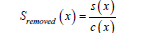
Drill core data is initially collected in ENVI files, which contain data cubes with reflectance values across a range of wavelengths. We referenced these cubes with the first column representing the depth of the drill core and the remaining columns indicating reflectance across the spectral bands. However, the raw drill core data often contains background noise and broad trends that can mask the key spectral features. To address this, we applied for each spectra continuum removal, a critical step that keeps spectral information by removing the general effects of the Planck curve and effects like water vapour and sensor specifics. The process involves fitting a smooth curve, or continuum, to the reflectance spectrum by using a convex hull approach. The convex hull creates an upper boundary that encapsulates the spectral data, providing a baseline over which other features are observed. By interpolating between the points of the convex hull, we generate a smooth continuum that represents the general trends in the data. The continuum removal technique involves dividing the original reflectance values by this interpolated continuum, effectively normalizing the spectrum and emphasizing unique spectral features. The equation for continuum removal using a convex hull can be described as:

Where:
S(x) is the original reflectance spectrum
C(x) represents the continuum derived from the convex hull and interpolation
S_removed(x) is the continuum-removed spectrum, with the background trends “flattened”

Figure 1 shows the data structure on a sample of the SGU dataset, where from the image-based reflectance datacube to a table with reflectance values per scan line to a training sample containing along the horizontal axis the spectral component and on the vertical axis the spatial component for the typically onemeter segment. The spatial resolution for the data was defined by the scan rate of the sensors, while the spectral component by the spectrometer resolution.

Figure 1:Overview of data processing process.

Model

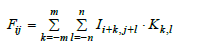
During the development, we established the advanced Neural Network CoreSmart2 which can be described in general as a Convolutional Neural Network (CNN). It is in general shown in Figure 2. CNN is known for its efficacy in handling spatial data such as images or spectral data with high robustness [30]. The CNN consist of convolutional and pooling layers, which utilize convolutional filters to extract features from input data, transforming them into randomized numerical values arranged in a grid. The architecture of the CNN developed follows a standard pattern. Initially, a Convolutional Layer (Conv2D) applies convolutional filters to the 250x250 input data, extracting spatial features. Mathematically, this can be described as:

Figure 2:CNN coreSmart2 layer workflow.

Where:
I_i+k,j+l is the input data, in this case the hyperspectral data of the drill core
K_k,l is the convolutional kernel
m,n represent the dimensions of the kernel

Next, the output of the convolutional layer is then passed through an activation function to introduce non-linearity. We use for activation functions is the Rectified Linear Unit (ReLU), defined mathematically as:

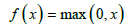
ReLU outputs zero for any negative input and retains positive values. This “rectifying” effect helps the network to learn complex patterns like our spectral-spatial feature sets without the vanishing gradient problem common in other activation functions like sigmoid or tanh. The linearity for positive inputs also reduces computation time. Subsequently, MaxPooling Layers (MaxPooling2D) downsample the output of the convolutional layer, reducing the spatial dimensions of the feature maps while retaining the most important information. This downsampling can be described mathematically as:

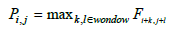
The equation indicates that for each position (𝑖, 𝑗), MaxPooling selects the maximum value within a given window size. We choose this downsampling as it reduces overfitting and computational complexity while preserving important spatial features. It also helps to make the network invariant to small translations in the input data, providing a degree of robustness. This combination of Convolutional and MaxPooling layers is repeated multiple times to extract increasingly abstract features from the input data to the final dimension of 64x64.

Following this, we incorporated Flattened Layer to convert the output from the pooling layers into a one-dimensional array, preparing it for input into a dense layer. The dense layers were responsible for combining the information from the previous layers to generate final predictions or classifications:

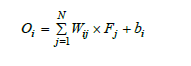
Where:
W_ij are the weights
F_j is the flattened array
b_i are the biases
O_i represents the output of the dense layer

The used weighted sum operation allows the model to learn complex relationships between the spectral-spatial features extracted by the Convolutional layers. Biases provided additional flexibility in the learning process, helped the model to converge more effectively. Additionally, a Dropout Layer was included to prevent over-fitting by randomly dropping a fraction of the connections between neurons during training. The Dropout operation is mathematically represented as:

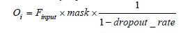
Where:
O_i represents the output of the dropout layer
F_input represents the input of the dropout layer

mask is a binary mask generated randomly, where each element is set to 0 with probability equal to the dropout rate, and to 1 with probability equals to 1 – dropout rate

dropout_rate is the probability of dropping out a unit By employing this model architecture, we aimed to leverage its ability to effectively extract features from the spectral-spatial dataset and facilitate accurate learning and predicting metal grades from the provided labels. In order to achieve this goal, we use 60% of the data as the training data, 20% of the data as the validation data, and the rest 20% as the testing data. We use the accuracy of the model which is defined as the ratio of correctly predicted instances to the total instances in the dataset to evaluate the model’s performance in predicting metal grades. We also defined metal grade based on the target metal percentage in the hyperspectral data cube.

To test the CoreSmart2 CNN we were using percentiles of the label records with metal grades derived from laboratory measurements. For example, the Cu05 percentile represents the top 5% of the copper content in the labelled dataset for all drill core samples which had also geochemical measurements. This means that the copper content in the Cu05 percentile contains the highest concentrations among all the copper grades. Table 3 below provides an overview of these percentiles and their corresponding thresholds in ppm for gold and copper and percent for iron. The authors are well aware that these thresholds for geological and mining technology-related questions are not suitable, for this article and in the interest of systematic tests we decided to divide the dataset into percentiles.

Table 3:Table of the metal grade percentiles and the thresholds used in this article.

Test setups

To understand the robustness and influencing factors on the CoreSmart2 neural network we run a couple of test setups, which are in the following described.
CoreSmart2 training to evaluate the influence of the spectral bands: To discern the impact of various spectral ranges on model performance, we trained CoreSmart2 for the VNIR/SWIR combined, SWIR alone and LWIR bands. The VNIR/SWIR (Visible Near-Infrared/Short-Wave Infrared) spans from approximately 400nm to 2500nm, SWIR (Short-Wave Infrared) operates from 1000 to 2500nm, and LWIR (Long-Wave Infrared) extends from 8000 to 14000nm. This strategy allowed us to thoroughly evaluate the impact of the band ranges as well the effects for instance involved in the combination of VNIR and SWIR like detector jumps on the CNN performance. By comparing the models trained on these different datasets, we sought to determine which spectral range provided the most accurate geochemical grade prediction.
CoreSmart2 model testing on different geological domains: To test the performance of the model on different geological domains and mineral exploration equipment’s set-ups we conducted additionally to the Auscope data assessment using hyperspectral data sourced from core scans conducted by the Geological Survey of Sweden (SGU). The SGU core scans were collected using different sensors than the Auscope dataset and they have different geographic characteristics. Specifically, we applied the model trained with SWIR data from Auscope to this test. The primary objective was to gauge the model’s performance across geological domains and with varying hyperspectral sensors. Pre-processing the SGU dataset into a similar spectral-spatial system like the Auscope data required the dimension reduction of the dataset but enabled us to probe the model’s adaptability and resilience.
CoreSmart2 model shuffle test to evaluate the spatial component: The shuffle test for CNN aims to identify the impact of changing spectral musters due to spatial changes in the datasets. That means the question of how much influence the location of spectral features in the pre-processed segment of one meter or a multiple of it has on the prediction results. For this we encompassed three key variations, the training images were along the spatial axis partitioned into increments of one pixel, segments of 10% or 25%, followed by the random shuffling of every partition along the spatial axis of the segment. So, all the spectral information was still in the segment present, but in a different sequence. The hyperspectral data utilized in this assessment was derived from SWIR core scans undertaken by Auscope in Australia. This test was aimed to shed light on the CNN’s capacity to effectively interpret and adapt to variations in structures across the individual segments used for training.
CoreSmart2 model spectral resampling test to evaluate impact of the sensor setup: To verify the impact of the usage of data from other hyperspectral sensors, the original training data, featuring a spectral resolution of 4nm, underwent resampling to intervals of 5nm. The hyperspectral dataset employed for this examination was sourced again from Auscope SWIR core scans. The focal objective of this test was to scrutinize the CNN’s dependency on the wavelength setup of the training data – getting the spectral resolution reduced. Our aim was to ascertain whether the model’s predictive accuracy hinged solely on the specific wavelength setup utilized for training, or if it performed the ability to generalize effectively to wavelength setups different to the training spectral setup. This analysis evaluated the CNNS’s adaptability and predictive capabilities across a coarser spectral setup.

The following chapter describes the results of the different test. The thresholds for the prediction were based in percentiles of the sample data and not based on operational or economic metal grades.

CoreSmart2 model training to evaluate the influence of the spectral bands
VNIR/SWIR: The results of the model trained with VNIR/SWIR hyperspectral data are presented in Table 4. The table provides an overview of the model’s performance in predicting the presence of copper (Cu), gold (Au), and iron (Fe) within the drill core samples. They indicate the model’s accuracy in classifying samples into two categories: Class 0 (below the grade threshold) and Class 1 (above the grade threshold) for each metal. The average accuracy across all metal grades is also provided for each mineral category.

Table 4:VNIR/SWIR model prediction results, shown is the accuracy of correct identification below and above the threshold in percent.

For copper classification (Cu), the VNIR/SWIR model demonstrates robust performance, achieving an average classification accuracy of 86.37%. Within this, Class 0 exhibits consistently higher accuracies across varying grades, indicating the model’s proficiency in discerning lower copper concentrations. Conversely, Class 1, representing above-threshold copper concentrations, showcases comparatively lower accuracies, suggesting potential challenges in distinguishing subtle variations in geological setups and copper grade detectability.

Similarly, for gold classification (Au), the VNIR/SWIR model attains an average accuracy of 84.64%. Notably, Class 0 manifests superior accuracies across different grades, underscoring the model’s effectiveness in identifying lower-than-threshold gold concentrations. In contrast, Class 1 performances indicate some difficulty in accurately classifying above-threshold gold concentrations, as evidenced by slightly lower accuracies. In the case of iron classification (Fe), the VNIR/SWIR model exhibits an average accuracy of 90.42%. Class 0 showcases consistent and high accuracies, indicative of the model’s proficiency in distinguishing below-threshold iron concentrations. Conversely, Class 1 again performances vary across different grades, with relatively lower accuracy predictions above the threshold of iron concentration.

SWIR: The results of the model that was trained SWIR hyperspectral data only are presented in Table 5. The table provides an overview of the model’s performance in predicting the presence of copper (Cu), gold (Au), and iron (Fe) within the drill core samples, similar to the VNIR/SWIR model training. For copper predictions (Cu), the SWIR model achieves an average classification accuracy of 86.15%. Then the gold predictions (Au), the SWIR model attains an average accuracy of 82.76%. In the case of iron classification (Fe), the SWIR model exhibits an average accuracy of 91.16%. For all three metals again the accuracy of the correct predictions of metal grade below the thresholds was higher than for the predictions above the threshold.

Table 5:SWIR model prediction results, shown is the accuracy of correct identification below and above the threshold in percent.

LWIR: The results of training the drill core model with LWIR hyperspectral data are presented in Table 6. For copper classification (Cu), the LWIR model achieves an average prediction accuracy of 89.76%. Again Class 0 consistently exhibits higher accuracies across varying grades, indicating the model’s proficiency in predicting copper concentrations below the threshold. For gold prediction (Au), the LWIR model attains an average accuracy of 85.95%. In the case of iron classification (Fe), the LWIR model exhibits the highest performance, with an average accuracy of 95.19%. Class 0 consistently demonstrates high accuracies, different to other cases here Class 1 predictions reach the same or nearly same accuracies as Class 0.

Table 6:LWIR model prediction accuracy, shown is the accuracy of correct identification below and above the threshold in percent.

Figure 3:The prediction accuracy (%) of copper for CoreSmart1 compared to Coresmart2 VNIR/SWIR, SWIR and LWIR models.

Figure 4:The prediction accuracy (%) of gold for CoreSmart1 compared to VNIR/SWIR, SWIR and LWIR models.

Figure 5:The prediction Accuracy (%) of iron for CoreSmart1 compared to VNIR/SWIR, SWIR and LWIR models.

Comparison among all three models: Figure 3-5 are demonstrating the overall prediction accuracy of VNIR/SWIR, SWIR, LWIR and mineral abundance-based predecessor model CoreSmart1 [8] for copper, gold, and iron grade. We used CoreSmart1 as the baseline for this comparison. In general, CoreSmart2 had a higher performance than the precursor model CoreSmart1, which after mineral abundance analysis used the mineral tables for the prediction.

For copper (Figure 3) the LWIR model had in mostly the highest accuracy in the predictions followed by the VNIR/SWIR model, and the SWIR model has the lowest accuracy among all three models. Especially with lower copper grades the SWIR and the VNIR/ SWIR systems performed better, the reason might be the typical clay features. A similar observation was made for gold (Figure 4), here the VNIR/SWIR setup performed apart from the highest gold concentrations best or similar to the LWIR bands. Using the SWIR bands alone with CoreSmart2 was still better than the CoreSmart1 predictor but in general significantly lower than the other band combination. For iron (Figure 5) all band combinations showed extremely good prediction accuracies, again outperforming the CoreSmart1 predictor in all cases. Also, the usage of the LWIR bands was most accurate for higher concentrations of iron.

CoreSmart2 model training on SGU data on very different geological domains

Performance on SGU data: The SGU dataset, all classification accuracies were around 50% or biased to one class only. As this identified that the model can’t be applied directly, we decided to retrain the models using the SGU testing dataset. The training of the CNN was performed with data and from Auscope and SGU, means across different geological domains and using different hyperspectral sensors to assess their generalizability and robustness in diverse geological settings. The evaluation of the SGU data is presented in Table 7.

Table 7:Metal grade prediction accuracy of SWIR Model, shown is the accuracy of correct identification below and above the threshold in percent.

For copper predictions (Cu), the model achieved an overall average accuracy of 87.67%. In the case of gold (Au), the model predicted with an overall average accuracy of 85.89%. For iron classification (Fe), the average accuracy of the prediction was 85.13%. Similar to the first test results the accuracies of the below threshold Class 0 have higher values across different grades, indicating the model’s effectiveness in identifying the absence of the metals is better than predicting the present above threshold value.

Comparison between auscope SWIR model and SGU SWIR model: We used the accuracy of metal grade prediction from the SWIR model from the first test as the benchmark to verify the performance of the included SWIR model. The comparison results are demonstrated in Figure 6-8. For all three metals over both geological regions trained CoreSmart2 achieved higher accuracy for higher metal grades of the Australian data than the Swedish. On lower metal grades the SGU SWIR model improved and got better accuracy than the Australian data. The most likely reason is the limited amount of training data, especially for higher metal grades in the SGU data. For the lower metal grades, the quality of the SGU labels might also have a positive impact.

Figure 6:Comparison of the prediction accuracy of copper grades between Australian and Swedish data sets using a CNN trained on both datasets.

Figure 7:Comparison of the prediction accuracy of gold grades between Australian and Swedish data sets using a CNN trained on both datasets.

Figure 8:Comparison of the prediction accuracy of iron grades between Australian and Swedish data sets using a CNN trained on both datasets.

CoreSmart2 model shuffle test to evaluate the spatial component

Testing result on shuffled data: The shuffle test conducted for the drill core model encompassed three distinct variations of the input data for the training of the CNN. This changed the spatial component in the spectral-spatial, each aimed at evaluating the model’s sensitivity to spatial variations within the training data. Hyperspectral data sourced from Auscope’s core scans in Australia facilitated this assessment by examining the impact of shuffling at different levels splitting into increments of 10% and 25%, as well as shuffling every pixel by row within the training images.

Shuffling every pixel by row within the training images achieved an average accuracy of 82.16% for copper (Cu), 78.21% for gold (Au), and 87.81% for iron (Fe). When the training images were split into increments of 10% and shuffled along the spatial axis, the resulting classification accuracies varied across different mineral grades. For copper (Cu), the model achieved an average accuracy of 82.35%. Class 0 consistently exhibited higher accuracies compared to Class 1, indicating the model’s proficiency in predicting better copper grades below the threshold than above. Similarly, for gold (Au), the model attained an average accuracy of 78.58%, with Class 0 displaying again better prediction accuracy. The iron (Fe) prediction was done with an average accuracy of 88.15%, with relatively stable accuracies across both classes.

Splitting the training images into increments of 25% and shuffling led to slightly different classification outcomes. The model achieved an average accuracy of 82.81% for copper (Cu), 79.11% for gold (Au), and 88.38% for iron (Fe). Notably, the accuracies for Class 1 in copper and gold classifications were slightly lower compared to the incremental splitting of 10%, suggesting a potential impact of spatial variations on model performance. Comparing the results, a shuffle along the spatial axis by every pixel resulted in slightly lower accuracies than compared to both coarser splitting variations, indicating a potential influence of pixel arrangement on the model’s sensitivity to spatial distributions (Table 8).

Table 8:Auscope shuffle SWIR training results, shown is the accuracy of correct identification below and above the threshold in percent.

sComparison between non-shuffled data testing result and shuffled data testing result: We used the accuracy of metal grade prediction from the SWIR model from the first test as the benchmark to verify the effect of shuffling along the spatial axis. Figure 9-11 show the comparison results. The non-shuffled data testing result has the highest prediction accuracy on average 5% more accurate than the shuffled data testing results for all three metals. The prediction accuracy for all types of shuffled data test results is extremely close, and 25% shuffled has the highest accuracy and overall pixel shuffled data has the lowest accuracy. Hence, we can conclude while there is a spatial relationship for each data cube of a drill core the CoreSmart2 neural network is also predicting spatially different located spectral similar features in the data cube but with slightly lower accuracy.

Figure 9:Comparing the prediction accuracy of copper grades on non-shuffled data testing and shuffled data.

Figure 10:Comparing the prediction accuracy of gold grades on non-shuffled data testing and shuffled data.

Figure 11:Comparing the prediction accuracy of iron grades on non-shuffled data testing and shuffled data.

CoreSmart2 model spectral resampling test to evaluate impact of the sensor setup

Spectral resampling test result: The results of the spectral resampling test for the drill core model are shown in Figure 12- 14. This test aimed to assess the impact of resampling the original training data, which had a spectral resolution of 4nm, into a spectral resolution of 5nm and 10nm. The SWIR-only data from the Auscope dataset were applied to the trained SWIR model from the first test.

Figure 12:The prediction accuracy of copper grade of 4nm, 5nm and 10nm spectrum resolution data.

Figure 13:The prediction accuracy of gold grade of 4nm, 5nm and 10nm spectrum resolution data.

Figure 14:The prediction accuracy of iron grade of 4nm, 5nm and 10nm spectrum resolution data.

For copper classification (Cu), the model using 5nm data achieved an overall average accuracy of 81.02%. Class 0 again consistently exhibited higher accuracies across varying grades, indicating the model’s proficiency in predicting grades below the threshold. In the case of gold prediction (Au), the model attained an overall average accuracy of 82.26%. For iron classification (Fe), the model exhibited an overall average accuracy of 89.61%. For the 10nm resampled data the accuracy was even lower and for lower thresholds the Neural Network was not capable to predict any longer correctly the metal grades.

Comapring the accuracy of metal grade prediction from SWIR model from first test with nominal spectral resolution of 4nm as the benchmark to verify whether changing the spectrum resolution of the data will affect the metal grade prediction results Figure 12- 14 show the comparison result. In general, the SWIR model with 4nm spectral resolution data can predict the metal grades more accurately than with 5nm spectral resolution data and 10nm spectral resolution data. With lower metal grades the prediction accuracy of the resampled data gets also lower, especially noticeable on iron, the decrease is stronger on the 10nm resampled data. Based on this result, we can conclude that changing the spectrum resolution of the data will affect the metal grade prediction accuracy and the higher spectrum resolution data yields more accurate metal grade prediction.

The principle of predicting metal grades directly from reflectance spectra

With the trained CNN it is possible directly to predict metal grades on the elementary level based on spectral data without mineral mapping based on spectral libraries or similar steps in between. Still, the physical principle on the molecular level of reflectance changes coursed by vibration and distortions in and around the molecular structure is used as it course the spectral signatures, the connection to the molecular structures like for instance OH-groups is not any directly used. Comparing the results from a precursor study for this development, where The Spectral Geologist (TSG) was used for mineral mapping and a CNN trained to predict grades based on mineral abundances [22] it shows the improvement of the accuracy results by using direct reflectance spectra.

The usage of the reflectance spectra directly to predict metal grades should offer a couple of advantages. The pre-processing with a modified continuum removal technique was helpful in producing a more suitable dataset for processing through the neural network. By enhancing the distinct spectral features, the neural network can easily extract the key features from the dataset which produces more accurate results. Moreover, the processed input data are showing also small absorption features in the resulting twodimensional datasets per drill core segment.

Second, the direct use of the reflectance spectra avoids the limitation of using spectral libraries, which in a geological setup – especially for larger areas – never can cover all mineralogical specimens with different patinas for instance from atmospheric and biological layering. Spectral libraries are all times collections of carefully curated spectral samples from the field or laboratory representing the range of the spectral variability for this mineral in limits. Furthermore, the established spectral classification methods – which have left infancy for a while [31] – are working on mathematical analysis of the spectra, reduction of dimensions, and band ratios. Quantitative approaches using parameters of specific absorption bands and similar measurements [8]. These methods are suitable for specific scenes and might require extensive fieldwork and ground sampling. This ground sampling is in the here presented trained CNN CoreSmart2 replaced by the usage of data from large drill core databases. Drill core scanning can be even with the variability of the core quality seen as collecting spectral data in a very controlled environment, with stabilized light sources and stabile correction to reflectance values. Additionally, smaller differences in the methodology are in more than one thousand kilometres of core a statistically covered variance which the neural network can work with. The label used geochemical Drill core databases like Auscope or the SGU database also cover most of the geological setups and deposit types of the region. Kutzke et al. [24] could show that the performance of the precursor to the here presented Neural network was capable of learning and predicting metal grades over a large geological domain, learned in one and applied in another. Unpublished tests of the authors of this article showed that the performance of the predictions is deposit type depending, it was possible to predict copper grade values correctly also outside of Australia for the orogenic belt of the Selenge in Mongolia, similar to the training used areas from Yilgarn Craton including the Eastern Goldfields Superterrane in Western Australia, the deposits in the Eastern Goldfields Superterrane, the Victorian goldfields, the Cobar district in New South Wales and others. Same time it was not possible to predict with good accuracies for instance copper grades based on spectral scans from the Las Bembas Mine in Peru due to the different geological settings and missing learning data. The mitigation for this problem is the implementation of additional reflectance spectra of core data with geochemical labels from the specific deposit as in this publication done with the SGU data, including banded iron deposits.

The general limitations of the developed CNN are in coverage of the geological domain or deposit types during the training process with enough labels and mean with enough segments with geochemical analysis. It is possible to integrate at any time new geological regions into the CNN and also to verify the usability by applying the model and checking on control labels performance, which should be in the range of the above-given accuracies. Other limitations are the commodities, which the CNN could be successfully trained on. While this publication shows for the introduction of the concept and the research on influencing factors and setups only results for copper, gold and iron other metals like uranium, lead, zinc and silver have been trained as well. There is also a model for nickel, but it needs to be noted that it covers only sulphidic nickel deposits and with a smaller number of labels. Summarizing the developed CNN has the capabilities to predict metal grades directly from reflectance-corrected hyperspectral data for most industrial metals and over a wide variety of deposits with the possibility to integrate via extended training further deposits and models.

Variability and robustness of the neural network

In a series of tests, the behaviour of the Neural Network under the influences of parameters related to sensor setup and data sources of the data were evaluated. By varying bands to use, sensor setups and even modifying the data of the individual one-meter segments in their spatial compositions we tested the robustness of the solution. Comparing the bands SWIR and VNIR/SWIR as a combination had similar performances, adding the VNIR range of 400 to 1000nm did not increase results. For operational reasons on drill core scanning that means that a SWIR system alone will perform well, in iron deposits the VNIR might be for the Fe2 and Fe3 separation in the mineralogy important, but for most applications, a SWIR sensor seems suitable. The usage of more expensive LWIR sensors can slightly improve the accuracy of the neural network predictions, especially when expecting higher concentrations of the metals. The biggest advantage of the LWIR is to see in applications of underground mining, where the reflectance sensors are limited or require higher efforts on the lamps. In this environment solutions like illumination with a thermal source or double data recording with and without thermal illumination are easier to handle. Unknown is how far the better results for higher concentrations of the tested metals are based on dominant quartz structures, which are by the LWIR sensor effectively mapped also in their variability while the SWIR can only indirectly deal with them.

Implementing more hyperspectral scans from a different geological domain – in this case, Sweden – was not only a model application. The neural network needed some additional training, which might have been a combination of different factors. On one hand, the dominant banded iron structures of the Swedish deposits were “new” to the AI, other hand the scanning and handling of the data different to the Auscope data with different sensors as well as different processing might have been the reason for that. The reflectance of the Swedish data was in some cases larger than the value 1, which points to methodological differences in the correction from at-sensor radiance to reflection. But after implementing the data from Sweden into the learning – together with the Australian data – the performance was nearly similar to Australia, which shows that the Neural network can use basic learning and implement additional data also from different regions and with different technical parameters to predict for the extended area, even the number of labels for this area is small.

One of the major uncertainties was how much the spatial component of the analysed drill core segments influenced the prediction of the Neural Network, which means if typical spectral features were moved spatially to another part of the 1m segment. This was tested with the randomized shuffle test and the results provided showed that the accuracy of class 0 remained stable, indicating its consistency in classifying low metal concentrations. The accuracy of metal bearing segments – class 1 – was reduced by a typical 2 to 5 percents for all types of spatially shuffled segment data similarly, but still had a reasonable learning performance, meaning different segmenting of data along the axis of the hole works as well as different segment sizes. This allows flexibility in the drill operation regarding the setup of the spectral scanning but points also to the usability of the neural network for other applications. For higher gold concentrations the spatial patterns had a larger impact, which implies that the model heavily relies on spatial patterns and variations in the data to effectively identify and classify gold concentrations. In contrast, the model can predict iron concentrations with higher accuracy even in the absence of strong spatial variations, which can be also seen on core samples, where iron is an all-overlaying feature quite often.

Resampling the spectral data from the core scan to a different resolution showed a decreasing accuracy on lower metal grades, meaning that dominant features can be predicted also on slightly different spectral sensors, while less learnable features are getting lost in the resampling of the spectral features. It was not tested how far the spectral resampling can be stretched and how much a different sensor setup impacts, but the tests with the Swedish data, which were scanned with an instrument with different spectral sampling showing, that training of such data can be supported by the basic learned model. Overall, the test results show the robustness of the Neural Network for the prediction of metal grades. When comparing the model’s performance in the different tests to the original train results, it became evident that the model exhibits flexibility and adaptability. Despite being trained on different data, the model consistently achieved competitive accuracy levels. This outcome underscores the Neural Networks robustness and ability to be applied to new datasets and provides and new way of using hyperspectral data in addition to existing industry-standard tools for minerals-based classification tools.

Potential application of the neural network besides drill core analysis

The Neural Network exhibited a consistent trend of accuracy across metal classes and with the above discussed robustness. As hyperspectral data in the SWIR range are commonly used also in other remote sensing applications like ore sorting, mine face applications, airborne and satellite data collection for geological and mineral mapping it will be interesting to investigate the usability of the Neural network for this scale. One challenge will be the generation of the spectral-spatial dataset to apply the Neural Network and to learn. As different to a mineral abundance analysis based on pixel, Kutzke et al. [24] also show that the predecessor of this neural network worked directly on the individual pixels of an airborne scene to predict copper grades, for the direct hyperspectral to metal grade prediction the spatial component need to be generated. This can be done by using the spectral signature of different pixels using various kernel structures. This kernel structures should represent the specific situation of the expected metal appearance; we tested combining neighbouring pixels but also cross sections through potential target areas. Here more research and verification of different scales of data will have to be done. The shown performance on the neural network on implementation of unknown data into the learning procedures showed that the system can be used for such datasets, for other scale date calibration experiments should be planned [32-34].

In conclusion, the Neural Network has demonstrated its efficacy in predicting directly based on hyperspectral reflectance data metal grades, surpassing existing industry-standard tools and showcasing improved accuracy to the predecessor neural network, which was based on mineral abundances. The model exhibited consistent proficiency in predicting grades of copper, gold, and iron. The SWIR region seems also for this technology a reliable dataset, while the LWIR region opens a wider range of applications in the exploration and mining operation. Furthermore, the Neural Network exhibited flexibility and adaptability, consistently achieving competitive accuracy levels across different datasets. Diverse geological contexts, different modelled sensor setups and variations in the spectral-spatial dimension of the data were implemented and their effect on prediction was quantified [35-37]. Despite limitations, the model demonstrated potential when trained on specific geological datasets, offering promising prospects for application within those contexts not only for drill core but also using other hyperspectral datasets for the detection of metal grades. Overall, the Neural network presents a promising approach for accurate metal prediction using hyperspectral data, with implications for various parts of the mining industry, but also with the potential to be adapted to other targets where hyperspectral data are used like for concentration mapping. Further research and refinement of the model’s training methodologies can unlock its full potential and expand its utility in other scale applications based for instance on airborne and satellite datasets.

The authors would like to thank the Geological Surveys of South Australia and Sweden for the support accessing and understanding the drill core and geochemical datasets.

This research was funded by Dimap together with support of the Hong Kong government under the ESS scheme – funding application S/E002/21.

All data used in this research are publicly available from AuScope and the state web portals of the relevant ministries of the Australian states. The Swedish data can be requested from SGU.

1. Vane G, Goetz AFH (1985) Proceedings of the airborne imaging spectrometer data analysis workshop (NASA-CR-176210). Jet Propulsion Laboratory, California Institute of Technology, United States.
2. Kruse FA, Lefkoff AB, Boardman JB, Heidebrecht KB, Shapiro AT, et al. (1993) The spectral image processing system (SIPS) - interactive visualization and analysis of imaging spectrometer data. Remote Sensing of Environment 44(2-3): 145-163.
3. Boardman JW (1998) Leveraging the high dimensionality of AVIRIS data for improved sub-pixel target unmixing and rejection of false positives: Mixture tuned matched filtering. In Proceedings of the Summaries of the Seventh JPL Airborne Geoscience Workshop; JPL: Pasadena CA USA, pp. 55-56.
4. Kruse F, Jodie B, Adam L, Young J, Young K, et al. (2000) The 1999 AIG/HyVista HyMap group shoot: Commercial hyperspectral sensing is here. Proceedings of SPIE - The International Society for Optical Engineering.
5. Acosta ICC, Khodadadzadeh M, Delgado TR, Gloaguen R (2020) Drill-core hyperspectral and geochemical data integration in a superpixel-based machine learning framework. IEEE Journal of Selected Topics in Applied Earth Observations and Remote Sensing 13: 4214-4228.
6. Buckingham WF, Sommer SE (1983) Mineralogical characterisation of rock surfaces formed by hydrothermal alteration and weathering-application to remote sensing. Economic Geology 78(4): 664-674.
7. Hunt GR, Salisbury JW, Lenhoff CJ (1971) Visible and near-infrared spectra of minerals and rocks. III. Oxides and hydroxides. Mod. Geol 2: 195-205.
8. Eichstaedt H, Tsedenbaljir T, Kahnt R, Denk M, Ogen Y, et al. (2020) Quantitative estimation of clay minerals in airborne hyperspectral data using a calibration field. Journal of Applied Remote Sensing 14(3): 034524.
9. Rast M, Nieke J, Adams JS, Isola C, Gascon F, et al. (2021) Copernicus hyperspectral imaging mission for the environment (Chime). Conference paper presented at the IEEE International Geoscience and Remote Sensing Symposium (IGARSS).
10. Młynarczyk A (2020) Using fieldspec ASD to create hyperspectral imaging. ResearchGate pp. 236-242.
11. Crowley JK, Brickey DW, Rowan LC (1989) Airborne imaging spectrometer data of the ruby mountains, Montana: Mineral discrimination using relative absorption band-depth images. Remote Sensing of Environment 29(2): 121-134.
12. Mohan BK, Porwal A (2015) Hyperspectral image processing and analysis. Current Science 108(5): 833.
13. Abbaszadeh M, Hezarkhani A (2013) Enhancement of hydrothermal alteration zones using the spectral feature fitting method in Rabor Area, Kerman, Iran. Arabian Journal of Geosciences 6: 1957-1964.
14. Bishop CA, Liu JG, Mason PJ (2011) Hyperspectral remote sensing for mineral exploration in Pulang, Yunnan Province, China. International Journal of Remote Sensing 32(9): 2409-2426.
15. Yousefi B, Sojasi S, Castanedo CI, Beaudoin G, Huot F, et al. (2016) Mineral identification in hyperspectral imaging using Sparse-PCA. In Thermosense: Thermal Infrared Applications XXXVIII 9861: 312-322.
16. Dramsch JS (2020) Chapter One - 70 years of machine learning in geoscience in review. Advances in Geophysics 61: 1-55.
17. Granian H, Tabatabaei, Hassan S, Asadi H, Carranza EJM, et al. (2015) Application of discriminant analysis and support vector machine in mapping gold potential areas for further drilling in the Sari-Gunay Gold Deposit, NW Iran. Natural Resources Research 25: 145-159.
18. Carranza EJM, Laborte AG (2015) Random forest predictive modeling of mineral prospectivity with small number of prospects and data with missing values in Abra (Philippines). Computers & Geosciences 74: 60-70.
19. Lobo A, Garcia E, Barroso G, Martí D, Turiel F, et al. (2021) Machine learning for mineral identification and ore estimation from hyperspectral imagery in tin-tungsten deposits: Simulation under indoor conditions. Remote Sensing 13(16): 3258.
20. Contreras C, Khodadadzadeh M, Tusa L, Ghamisi P, Gloaguen R (2018) A machine learning technique for drill core hyperspectral data analysis. In 2018 9^th Workshop on Hyperspectral Image and Signal Processing: Evolution in Remote Sensing (WHISPERS) pp. 1-5.
21. Liu C, Wang W, Tang J, Wang Q, Zheng K, et al. (2023) A deep-learning-based mineral prospectivity modeling framework and workflow in prediction of porphyry-epithermal mineralization in the Duolong Ore district, Tibet. Ore Geology Reviews 157: 105419.
22. Eichstaedt H, Ho CYJ, Kutzke A, Kahnt R (2022) Performance measurements of machine learning and different neural network designs for prediction of geochemical properties based on hyperspectral core scans. Australian Journal of Earth Sciences 69(5): 733-741.
23. Prado EMG, de Souza Filho CR, Carranza EJM (2023) Ore-grade estimation from hyperspectral data using convolutional neural networks: A case study at the olympic dam iron oxide copper-gold deposit, Australia. Economic Geology 118(8): 1899-1921.
24. Kutzke A, Eichstaedt H, Kahnt R (2022) Potential of hyperspectral-based geochemical predictions with neural networks for strategic and regional exploration improvement. Australian Journal of Earth Sciences 69(8): 1197-1206.
25. AuScope (2019) National Virtual Core Library (NVCL).
26. Schodlok MC, Whitbourn L, Huntington J, Mason P, Green A, et al. (2016) HyLogger-3, a visible to shortwave and thermal infrared reflectance spectrometer system for drill core logging: functional description. Australian Journal of Earth Sciences 63(8): 929-940.
27. SGU (2020) Drill Core Scanning at SGU. Sveriges geologiska undersökning, SGU.
28. Liljenstolpe C, Hamberg R, Selbach H, Larsson D, Abrahamsson S (2023) Statistics of the Swedish Mining Industry 2022 (Periodiska publikationer 2023:2). Geological Survey of Sweden.
29. EURARE (2013) REE mineralisation in Sweden.
30. Alex K, Ilya S, and Hinton GE (2012) ImageNet classification with deep convolutional neural networks. In Proceedings of the 25^th International Conference on Neural Information Processing Systems - Volume 1 (NIPS'12), Lake Tahoe, Nevada. Curran Associates Inc, Red Hook, NY, USA, pp. 1097-1105.
31. Vishnu S, Nidamanuri RR, Bremananth R (2012) Spectral material mapping using hyperspectral imagery: A review of spectral matching and library search methods. Geocarto International 28(2): 171-190.
32. Agrawal N, Govil H (2023) A deep residual convolutional neural network for mineral classification. Advances in Space Research 71(8): 3186-3202.
33. Perozzi ACL, Gloaguen E, Blouin M (2017) Machine learning as a tool for geologists. The Leading Edge 36(3): 215-219.
34. (2019) Commonwealth Scientific and Industrial Research Organisation (CSIRO), HyLogging.
35. Huston D, Mernagh T, Dulfer H, Skirrow R (2013) Geology of critical commodities, and Australia's endowment and potential. In Critical commodities for a high-tech world: Australia's potential to supply global demand. Geoscience Australia.
36. JICA (2013) Final report on the comprehensive study of the mining sector in the Republic of Kazakhstan.
37. Sun Y, Sun, Z, Lv H (2019) Deep convolutional neural network for mineral classification using hyperspectral imaging. IEEE Transactions on Geoscience and Remote Sensing 57(1): 400-410.