Tool Wear Classification for Conical Picks Using Acoustic Fourier Spectra Magnitude

Underground coal mine workers who operate continuous mining machines rely on many cues to determine tool wear. This skill is difficult to train and proximity to the mining interface is a hazard to the machine operators. To create safer conditions for machine operators, an acoustic classification method for determining tool wear is proposed. To demonstrate this technique, a concrete sample is cut with conical picks of different wear levels using a linear cutting machine and the acoustic data is recorded for classification experiments. The differences in acoustic frequency spectra are highlighted and classification of short segments of the recorded acoustic data, less than 200 milliseconds in duration, is demonstrated using three popular classification techniques: the K-nearest neighbors classifier, the support-vector machine classifier, and the multi-layer perceptron classifier. The performance of these techniques is compared, and the effects of segment size and down sampling are examined. Of the tested methods, the support-vector machine gives good performance with little complexity. This technology could aid operators in performing their roles from a safer distance, alerting them to worn tool conditions in real time.

Keywords:Acoustic classification; Tool wear; Conical picks; Underground mining; Support-vector machine; K-nearest neighbours; Multi-layer perceptron classifier; Fourier transform; Vibration

Abbreviations: FTE: Full Time Equivalent; NIOSH: National Institute of Occupational Safety and Health; kHz: kilohertz; dBA: A-Weighted Decibel; KNN: K-Nearest Neighbours; SVM: Support-Vector Machine; MLP: Multi-Layer Perceptron; RBF: Radial Basis Function

Underground mining safety has not improved over the last decade, with the average annual rate of fatalities per 100,000 Full Time Equivalent (FTE) workers being roughly 24 from 2011 to 2022 [1]. In the literature review conducted by Sari et al. [2] it is noted that younger, less experienced miners are at greater risk of suffering a disabling injury [2]. On the other hand, for older and more experienced miners, the high levels and long duration of exposure to the hazards inevitably leads to problems like hearing loss [3], or other diseases such as black lung, a serious lung disease caused by exposure to coal dust, which can be fatal [4]. Some examples of dangers in the underground mine environment include tunnel collapse, explosive gasses [5], high temperatures [6], exposure to diesel particulate [7], and the crush hazards caused by the machines used for the operation [8]. Machine operators in underground coal mines are particularly at risk, as they must remain near the cutting interface to pick up cues from machine and the environment to monitor cutting conditions [9]. Workplace accidents caused by these hazards are problematic and they lead to loss of productivity, worker injury, and loss of life [10]. The National Institute for Occupational Safety and Health (NIOSH), recommends removing workers from hazardous locations as the best form of risk reduction in general [11].

Aiding operators with improved sensors for tool wear detection can help them perform their role from a greater distance to the cutting interface and reduce their risk from dust exposure as well as from the immediate dangers at the cutting interface. Experienced operators are an invaluable resource, as they hold the experience gained after years of dealing with hazardous conditions [9]. Operators are known to rely on many cues, including visual, acoustic, and vibrational. This suggests a sensor can measure these cues. Acoustic sensors can operate with a quick, less than one second, response time and detect changes in material type and tool wear in many domains [12-15]. When comparing acoustic, visual, and vibrational cues for tool wear, acoustic detection of tool wear has the advantage over visual detection in that it does not require a clear line of sight to the cutting interface, which is often in a hazardous location near the machine [9]. Alternatively, vibrational cues require direct contact with the cutting process, which requires a more robust sensor design compared to an acoustic sensor which is placed further away. For these reasons, using acoustic data for objective tool wear classification from a distance is investigated in this work. Any technology that is employed in this domain must be well suited for the task it is designed to perform, or else its adoption is unlikely [8]. By providing objective, real-time data to human operators, the proposed technology can help operators make objective decisions regarding shutting down operations for cost-saving maintenance or continuing work. Automating tool wear detection can also allow machine operators to focus on other aspects of machine operation, increasing their productivity. Automation also enables the collection of data that could be analysed for trends in tool wear during operation.

The rest of this article is outlined as follows. In the Background section, the application background and previous work used to guide this study are discussed. The Methods section follows, and it gives a detailed description of the experimental equipment, classification methods, and metrics for comparing classification performance. After that, the Results section lists the notable results. Then, a Discussion section is given, which states the merits of the tested methods and provides recommendations for implementation. Finally, a conclusions section summarizes the work and its relevance considering the target application.

In the black lung study by Colinent, the author notes that much effort has been given to dust mitigation. Strategies include minimizing dust generation, preventing dust from circulating, removing dust from circulation, diluting dust concentration, use of barriers and ventilation direction to reduce worker expo- sure, and maintenance of these systems [4]. The idea of removing workers from hazardous zones is supported by the general advice given by NIOSH in their hierarchy of controls [11]. In order to remove workers from the hazardous zones, they must be enabled to perform their roles from more remote locations.

Considering that experienced human operators can detect tool wear using acoustic cues suggests that enough relevant information can be captured within the typical human hearing range. A study on occupational hearing loss in underground mines reported that the type of hearing loss experienced by underground coal miners indicates a noise frequency below 6kHz and a noise intensity around 90dBA [3]. This work aims to capture these low-frequency and high-intensity acoustic emissions for classification.

As early as the 1990s, methods that consider the total volume of the acoustic emissions, the count of peaks and valleys in the signal, and the changes in signal spectra have been researched [16,17]. Proper preprocessing is important. In underground mining, the rock-cutting system can lose mass as tools are worn, resulting in a non-stationary dynamic system. Fast Fourier transform based preprocessing of a small window of signal and subsequent classification with a support-vector machine has shown to be an effective method for robust classification of non-stationary dynamic systems [18]. Other preprocessing techniques for similar problems include wavelet and Empirical Mode Decomposition. Wavelet preprocessing combined with machine learning has been used with success in recent years [19-21]. Empirical Mode Decomposition has demonstrated vibration classification for tool wear in other domains [22-24]. Fast Fourier spectra magnitude based preprocessing with normalization is chosen for its timeinvariant properties, small number of hyperparameters, and known effectiveness across domains [25,26].

Both wavelets and Empirical Mode Decomposition are timevariant. The wavelet transform is known to be very sensitive to small-time translations [27]. With wavelets, this can be mitigated by measuring the average energy for a continuum of offsets and using those values as the feature vector for classification [28]. Similar processing would be needed for Empirical Mode Decomposition. Another option is to register the signal in the time domain to an event, such as contact with the material. The choice of preprocessing methods is motivated by the idea that different tool wear levels in a conical pick will produce different acoustic emissions with different Fourier frequency spectra magnitude for a given material. This is verified by analysing objective differences in statistical distributions of the frequency spectra magnitudes for the tested categories. To leverage these differences, different classification techniques are employed and compared. These methods and how they are compared are described in the next section.

A homogeneous concrete sample is cut using the Linear Cutting Machine at the Earth Mechanics Institute at the Colorado School of Mines, shown in Figure 1, and capable of testing with many cutting tools [29]. Hydraulic actuators move the rock box for positioning and cutting. The rock sample in this experiment is a solid block of concrete. This is a homogeneous material that will isolate the changes in tool wear. Additional equipment consisting of a dust shroud and vacuum sample collection system was used for a simultaneous study on dust generation, but not for this study. Forces are recorded using integrated load cells in the coupling between the tool and the frame. The acoustic signals for this experiment were recorded from the camcorder used to capture Figure 1 at a sample rate of 44.1kHz. Then, the data is categorized by tool wear condition. The different tool wear levels are shown in Figure 2. The tool tips have been artificially worn with a lathe to a spherical shape to approximate even wear. They vary in diameter and have been chosen to represent new, moderately used, and worn tooltips. The new tool is unmodified and has a diameter of 3.71mm, the moderately used tool has a diameter of 17.9mm, and the worn tool has a diameter of 27.5mm.

Figure 1:The linear cutting machine at the earth mechanics institute of Colorado School of Mines.

Figure 2:The tips of the conical picks with different wear levels used for the experiment.

The sample is cut by layers, with each layer consisting of several lines spaced roughly three centimetres apart. The cutting speed is set to 10 inches per second and penetrations of 1.5 and 2.0 inches are used. For each wear category, four lines are collected for both penetrations. To reduce the edge effects of the experiment, like the differences in impulse response between the linear cutting machine and the sensor, the recording of each line is trimmed to 6 seconds, starting shortly after the bit hits the material. The data is chopped into small segments of 20, 40, 60, 80, 100, and 200 milliseconds in duration. The segments are allowed to overlap by 50%, and this yields roughly 480 samples for the 100-millisecond case and 4800 samples for the 20-millisecond case for each wear category.

The fast sampling rate of the microphone, 44.1kHz, means that even short segments, dozens of milliseconds in duration, will have thousands of data points. Reducing input dimension via down sampling after low pass filtering will preserve low frequency data while leading to faster processing for the classification algorithms and eliminating additional aliasing. These segments also have a Hamming window applied to enforce periodic assumptions of the Fourier based preprocessing [30]. Longer signal windows will yield more resolution in the frequency domain up to the sampling frequency while higher sampling rates offer slightly increased resolution but over a wider frequency range. This study compares the effect on classification performance from both down sampling and window length.

Method performance is rated using the F1 score, which penalizes false positives and false negatives, by generating a distribution of scores and comparing the distributions [31]. The confusion matrices of the classifiers are also examined to understand how the classifier is performing [32]. Each window size data set is divided randomly in a 70:30 test train split 40 times to collect statistical distributions of the scores for each classification method when using a small sample for training data. The preprocessing and classification methods are described in more detail below.

Preprocessing

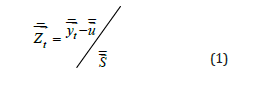
After filtering, down sampling, and splitting the data into small segments, the input to each of the classification algorithms is a vector of floating-point numbers which represents a small segment of the audio recording from the cutting experiment. Any segment of the data, starting at time t, is denoted as . This vector has consecutive samples of the time domain signal starting at time t and ending at the end of the window duration offset by the start time. The first preprocessing step is to multiply this vector elementwise with a Hamming window, and the new vector is given as:. The exact choice of window function has subtle effects on the algorithm performance, but in general the window function serves to reduce spectral leakage, or aliasing [33].

After the window is applied, the Fourier based preprocessing begins. The datasets are split 70:30 into the test and train sets. The normalized data is denoted as , and it is calculated as:

where both subtraction and division are performed elementwise, u represents the vector of mean values for each dimension in the training set, and_s  represents the vector of standard deviations for each dimension in the training set. The distributions of frequency spectra magnitudes and time domain wave- forms for each wear category are shown in Figure 3. The Fourier transform data has most of its energy below 4kHz. The higher frequency data has smaller variance compared to the lower frequency data. The time domain data is roughly shaped like the window function. Transforming the time domain data into the frequency domain highlights the changing modes between the categories. These differences in resonant frequencies are made more apparent after normalization. During each classification experiment, the test data is normalized according to the distribution of the training set.

Figure 3:The natural distribution of frequency spectra magnitude and time domain data of each wear category for data.

Before invoking any classifiers, objective differences in acoustic spectra across wear categories can be shown by performing a classic two-sided Welch-Satterthwaite t-test on each frequency bin [34]. The results of this test and the normalized frequency spectra magnitude distributions for each wear category are shown in Figure 4. In the left column, the mean value and the standard error of the mean are shown for the collected data. In the right column, the results of a t-test for each bin for each pair of categories are shown. It is known that operators use acoustic signals to determine cutting conditions, and this figure demonstrates significant, p<0.001, differences across tool wear categories for most frequency bins. Even though the higher frequencies have less energy, their differences are still significant due to their low variance. The exact changes will depend on the machine and the entire set of cutting conditions, but for a given environment, these differences can be observed and detected. The classification techniques discussed in the next section use these differences to determine the wear category of a given sample based on the training data.

Figure 4:The mean frequency spectra magnitude after normalization for each wear category and a comparison between the categories for significant differences.

Classification

These data splitting, preprocessing calculations, and classification techniques are computed using the scikit-learn, a.k.a. sklearn, library [35]. The library supports many classification and regression methods and facilitates rigorous comparison. For this study, the support-vector machine technique is compared with a simpler method and a more sophisticated method to investigate classifier efficiency. The simpler method is the k-nearest neighbors classifier. The k-nearest neighbor technique works by comparing the input sample to its memory of the k closest training samples, and the most popular class is elected as the output. The more sophisticated method, the multi- layer perceptron classifier, works by training a network of artificial neurons to develop a series of vector transformations which results in accurate classification. Meanwhile, the support-vector machine aims to find a separating hyperplane in a transformed version of the data.

To measure the performance of the chosen algorithms, the F1 score is used to evaluate the classification results. There is an inherent trade-off between precision and recall in practical classifiers [36]. The F1 score is the geometric average of precision and recall and serves to evaluate overall performance. More detailed descriptions of the individual classification algorithms follow below.

K-nearest neighbors

The non-parametric K-nearest neighbors approach is used in classification and regression [37]. The K-nearest neighbors classifier aims to predict the class label, gt of future data point x₀ on the predetermined q classes given a set of p labeled classes {(x_t, g_t), t ∈ 1 . . . p} [38]. In order to obtain the class label for x₀, the K-Nearest Neighbor (KNN) classification algorithm searches for the sample’s K closest neighbors and then assigns the class of the majority. The selection of K and the distance measure used are the two factors that have the biggest impact on a KNN classifier’s performance [39]. Without prior knowledge, Euclidean distances are typically used by the KNN classifier as the distance measure. These distances are simple to compute and if the data categories are distinct, then this method will work well. The Euclidean distance and K=5 are used for this study, with larger values of K giving similar results.

Support-vector machine

The fundamental goal of the Support-Vector Machine (SVM) is to build a separation hyperplane that best divides data examples into two classes while maximizing the minimum distance between points and the separation hyper-plane [40]. Support-vector machines employ the structural risk minimization [41] concept and seek to achieve zero misclassification error while reducing the model’s complexity. The problem statement and solution of its dual via Karush-Kuhn-Tucker conditions [42] is omitted here for brevity. For discussion, the decision function of the two-class supportvector machine is listed here:

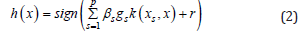
where sign returns 1 if the input is greater than zero, p is the number of support-vectors, β_s and g_s are weights, and k(x_s, x) is the kernel mapping of the support-vector x_s and the input, x, and r is a bias term. The kernel function is able to compare the input to the chosen support vectors in a space that highlights their differences.

The SVM is a binary classifier by nature, however many interesting problems are multi-class (q-class) [43]. Hence a multiclass SVM approach must be adopted in that regard. In this study, a one-against- one approach [44] is employed. This approach trains q(q-1) binary classifiers to distinguish between two classes. The final output is the class that receives the most votes from the binary classifiers. The coefficients calculated during training are considered optimal for the given data. The SVM requires a roughly similar number of computations as the KNN but takes extra steps to make the data more separable through the kernel function. The Radial-Basis function is used here for the kernel, as it can make nonlinear separations.

Multi-layer perceptron classifier

A specific type of feed-forward artificial neural network is the Multi-Layer Perceptron (MLP) and it is well-known for its stability, usability, and relatively modest structure in tackling some tasks when compared to other structures [45]. An MLP classifier analyzes the relationship between input and output in a set of p-labeled classes. An input layer, several hidden layers, and an output layer make up the network topology of MLP [46]. Processing nodes known as neurons make up each layer, with each neuron connected to all neurons in the previous layer. Each neuron receives weighted inputs with a bias value, which are then transformed and processed by a nonlinear activation function [47]. The hidden layer’s output is shown in the following:

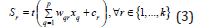
where the activation function is represented by t(•); the bias of the r^th hidden units is represented by c_r; the inputs and weights between the input and hidden layer are represented by x_q and w_qr, while S_r is the hidden layer’s output. Activation functions come in a variety of forms, including logistic sigmoid, softmax, hyperbolic tangent, and rectified linear unit functions [48]. The output layer consists of one neuron for each class, and the output is the probability that the input belongs to that neuron’s respective class.

The coefficients for the network are trained in an iterative fashion by examining the gradient of performance with respect to each one. This forward pass and back-propagation process is repeated until the network finds a solution or the necessary number of iterations have been completed [49]. This type of training requires a balance of many factors to be successful; but once trained, the network can classify samples with a roughly similar number of computations as the other techniques depending on the network size. The rectified linear unit activation function and a network of two hidden layers equal in size to the input dimension is used here, with more hidden layers giving similar results.

The mean F1 scores are plotted against the window lengths for each of the tested methods at each of the tested down sampling factors. In the following figures, the F1 score of a method is significantly greater than another method if the median score is above the max score of the other method. This comparison method is slightly more conservative but more visually straightforward than comparing each score in the collected distribution, as recommended in [31]. Classifier performance was greater with longer window lengths and increased sampling rates, or lower down sampling factors.

The K-nearest neighbors classifier performance is shown in Figure 5. Using K=5 gave slightly better performance than other values, but this method performed the worst overall. Increasing window length gave better performance for this method, and down- sampling had little effect for larger window lengths. The F1 score only increased a small amount when using the 0.2 second window compared to the 0.1 second window. The support-vector machine classifier performance is shown in Figure 6. This is a low hyperparameter method that performs very well and does so efficiently. With this method, performance trends are better with longer window length and higher sampling rates, or less down sampling, for the experiment. Increasing window length gave a better performance for the number of variables introduced compared to increasing sampling rates. Using a window length of 0.2 seconds gave the best performance of for all down sampling levels, and the performance was similar for samples with less down sampling.

Figure 5:The mean F1 score and standard deviation for K-nearest neighbors method.

Figure 6:The mean F1 score and standard deviation for the tested support-vector machine method.

The multi-layer perceptron classifier performance is shown in Figure 7. This method has the power to classify data very accurately for samples similar to its training data. Different network sizes are tested to achieve maximum performance. This method scores similarly to the support-vector machine but uses more resources. Both longer window lengths and higher sampling rates, or less down sampling, increased performance. Increasing window length gave better performance for the number of variables introduced compared to increasing sampling rates. Using a window length of 0.2 seconds gave the best performance of all down sampling levels, and the score tapered to about 0.90.

Figure 7:The mean F1 score and standard deviation for the tested multi-layer perceptron methods.

Looking at the confusion matrices for the different types of classifiers generally showed that most of the confusion was between the moderate and worn categories of bits, suggesting that these two categories have responses that are more similar to each other than to the new category. A sample confusion matrix for a SVM classifier experiment is shown in Table 1, it is representative of most of the other classifiers too. The table shows data for the concrete sample using a 70:30 test train split and with fast Fourier transform preprocessing of a 100-millisecond window. The table shows that there is about twice as much confusion between moderate and worn categories as there is between new and the other two wear categories. This indicates that determining wear to a fine degree may be difficult with acoustic emissions alone.

Table 1:Confusion matrix for acoustic wear classifier, normalized by true class size.

It is well known that changes in tool wear produce changes in vibrational response across many domains. This fact is also true in the case of underground mining. Human operators use sound cues as one of the means of assessing tool wear during operation. The operators have many duties, and this skill can be difficult to train, since the process is subjective. By providing operators a means to perform some of these duties from a safer position, their exposure to risks at the mining interface can be reduced [9]. This work proposes the addition of objective acoustic data collection and analysis to aid in tool wear classification. When using methods like the ones described in this work, the cutting conditions must be taken into account. For example, cutting different materials can also produce different modal responses as well as cutting at different speeds, penetrations, and with different tool geometries. The operator’s ability to deduce changes in wear in different materials comes from experience in cutting those materials with tools at different wear levels. Likewise, to successfully apply this technique, data would need to be captured and analyzed for different cutting conditions.

When comparing the methods for implementation in the application, the support-vector machine would be an efficient classifier to use, as it scores as well as the multi-layer perceptron classifier, but has reduced computational complexity. The results also indicate that longer sample times, which give increased resolution for the sampled frequencies, provides better classification performance than using an increased sampling rate for a shorter duration considering the number of variables introduced. With a window of 0.2 seconds, the tested sampling rates had similar performance. At this sample length, the input dimension is large, especially when little down sampling is used. Use of larger samples was computationally infeasible for the equipment and would also have reduced the number of samples available in the data set. The good performance of signals with long duration and down sampling implies that lower frequencies are of particular interest for tool wear classification in rock cutting. The code and data used for this work are available at: https://github.com/Fworg64/concrete tool wear.

After classification, human operators could be alerted to the anomalous conditions to allow them to make a decision to either stop the operation for further diagnostics or continue cutting if they know from experience what could be causing a false positive or how long to extend the current operation. Also, this technology that can monitor tool wear in an objective manner would provide a mechanism to monitor the performance of human operators. This can help operators and other stakeholders identify areas where they can improve. It can also be used to assist in training and help to identify risky operations. Either way, the feedback could be collected from a greater distance, reducing the operator’s exposure to dust and other hazards.

To implement this technology, only a simple and low-cost microphone would need to be placed near the cutting interface to detect the mode shifts associated with changing tool wear. These devices are low power, low cost, and very portable, making them well suited for the mining environment. However, since the signal is only collected from one or maybe several points, it is unlikely that this technology could predict which tools are worn on the drumhead. Also, interference from nearby operations which are producing noise could also affect the accuracy of this method were it to be deployed to an active mine. Ultimately, this technology could assist operators in performing their role from a greater distance and provide a level of objective feedback that is not currently present.

This paper showed a method for classifying the different acoustic signals generated by conical picks of different wear levels cutting into a controlled concrete sample. The changes in tool mass and geometry lead to excitation of different modes, which can be detected and classified by the tested methods after appropriate preprocessing. Of the tested methods, the support-vector machine using long duration samples that are down sampled to an appropriate dimension, like 200 milliseconds and 4 times down sampling, performs well and is computationally efficient. Acoustic emissions are currently processed by human operators with many duties. By automatically classifying the acoustic emissions, operators can be enabled to perform their role from a greater distance. This way they can avoid hearing damage, harmful dust, and machine proximity while being able to focus on their many other duties. With sufficient data collection, this classification can be performed with a microphone and an embedded processor.

Special thanks to AliseH and Tivali24 for contributions to the python code for running the experiments and displaying the data. Special thanks to Syd Slouka for helping run the experiments and to Carson Malpass for helping design mounts for acoustic sensors.

1. (MSHA), M S H A, NIOSH Mine and Mine Worker Charts: Fatality Rates for Operators in Underground Coal Mines.
2. Sari M, Duzgun HSB, Karpuz C, Selcuk AS (2004) Accident analysis of two Turkish underground coal mines. Safety Science 42(8): 675-690.
3. lknur E (2022) Investigation of occupational noise-induced hearing loss of underground coal mines. Mining, Metallurgy and Exploration 39: 1045-1060.
4. Colinet JF (2020) The impact of black lung and a methodology for controlling respirable dust. Mining, Metallurgy & Exploration 37: 1847-1856.
5. Juganda A, Pinheiro H, Wilson F, Sandoval N, Bogin GE, et al. (2022) Investigation of explosion hazard in longwall coal mines by combining CFD with a 1/40th-scale physical model. Mining, Metallurgy and Exploration 39: 2273-2290.
6. Cinar I, Ozsen H (2020) Investigation of climatic conditions in underground coal mining. Mining, Metallurgy and Exploration 37: 753-760.
7. Bugarski AD, Vanderslice S, Hummer JA, Barone T, Mischler SE, et al. (2022) Diesel aerosols in an underground coal mine. Mining, Metallurgy and Exploration 39: 937-945.
8. Swanson LTR, Bellanca JL (2019) If the technology fits: an evaluation of mobile proximity detection systems in underground coal mines. Mining, Metallurgy and Exploration 36: 633-645.
9. Bartels JR, Jobes CC, Ducarme JP, Lutz TJ (2009) Evaluation of work positions used by continuous miner operators in underground coal mines. Proceedings of the Human Factors and Ergonomics Society 53(20):
10. Sensogut C, Kasap Y, Oren O (2021) Investigation of work accidents in underground and surface coal mining activities of western lignite corporation by data envelopment analysis (DEA). Mining Metallurgy and Exploration 38: 1973-1983.
11. (2015) NIOSH: Hierarchy of controls. Centers for Disease Control and Prevention, USA.
12. Zakeri V, Hodgson AJ (2017) Classifying hard and soft bone tissues using drilling sounds. In: Proceedings of the Annual International Conference of the IEEE Engineering in Medicine and Biology Society, EMBS, pp. 2855-2858.
13. Zhong ZW, Zhou JH, Win YN (2013) Correlation analysis of cutting force and acoustic emission signals for tool condition monitoring. In: 2013 9^th Asian Control Conference, ASCC 2013, Turkey.
14. Rad JS, Zhang Y, Aghazadeh F, Chen ZC (2014) A study on tool wear monitoring using time-frequency transformation techniques. In: Proceedings of the 2014 International Conference on Innovative Design and Manufacturing, ICIDM, Canada, pp. 342-347.
15. Zakeri V, Arzanpour S, Chehroudi B (2015) Discrimination of tooth layers and dental restorative materials using cutting sounds. IEEE Journal of Biomedical and Health Informatics 19(2): 571-580.
16. Tan CC (1992) Monitoring of tool wear using acoustic emission. In: Singapore International Conference on Intelligent Control and Instrumentation-Proceedings 2: 1063-1067.
17. Kakade S, Vijayaraghavan L, Krishnamurthy R (1995) Monitoring of tool status using intelligent acoustic emission sensing and decision based neural network. In: IEEE/IAS International Conference on Industrial Automation and Control, Proceedings, India, pp. 25-29.
18. Xu L, Zhou Y (2016) Fault diagnosis for BLDCM system used FFT algorithm and support vector machines. In: 2016 IEEE International Conference on Aircraft Utility Systems (AUS), China, pp. 384-387.
19. He Q (2013) Vibration signal classification by wavelet packet energy flow manifold learning. Journal of Sound and Vibration 332(7): 1881-1894.
20. Sadegh H, Mehdi AN, Mehdi A (2016) Classification of acoustic emission signals generated from journal bearing at different lubrication conditions based on wavelet analysis in combination with artificial neural network and genetic algorithm. Tribology International 95: 426-434.
21. Skariah A, Pradeep R, Rejith R, Bijudas CR (2021) Health monitoring of rolling element bearings using improved wavelet cross spectrum technique and support vector machines. Tribology International 154: 106650.
22. Xu T, Feng Z (2009) Tool wear identifying based on EMD and SVM with AE sensor. In: ICEMI 2009 - Proceedings of 9^th International Conference on Electronic Measurement and Instruments, China, pp. 2948-2952.
23. Nie P, Xu H, Liu Y, Liu X, Li Z (2011) Aviation tool wear states identifying based on EMD and SVM. In: Proceedings of the 2011 2^nd International Conference on Digital Manufacturing and Automation, ICDMA 2011, China, pp. 246-249.
24. Zhan SS, Min H, Le Y (2014) Using EMD to extract characteristic values of the tool vibration signals. In: Proceedings - 2014 6^th International Conference on Measuring Technology and Mechatronics Automation, ICMTMA 2014, China, pp. 799-802.
25. Xu L, Zhou Y (2016) Fault diagnosis for BLDCM system used FFT algorithm and support vector machines. In: IEEE/CSAA AUS 2016: 2016 IEEE/CSAA International Conference on Aircraft Utility Systems.
26. Harlianto PA, Setiawan NA, Adji TB (2022) Combining support vector machine-fast fourier transform (SVM-FFT) for improving accuracy on broken bearing diagnosis. In: 2022 5^th International Seminar on Research of Information Technology and Intelligent Systems, ISRITI 2022, Indonesia, pp. 576-581.
27. Yen GY, Lin KC (1999) Wavelet packet feature extraction for vibration monitoring. In: Proceedings of the 1999 IEEE International Conference on Control Applications (Cat. No.99CH36328), USA, 2: 1573-1578.
28. Baccar D, Sffker D (2015) Wear detection by means of wavelet-based acoustic emission analysis. Mechanical Systems and Signal Processing 60: 198-207.
29. Thyagarajan MV, Rostami J (2024) Study of cutting forces acting on a disc cutter and impact of variable penetration measured by full scale linear cut- ting tests. International Journal of Rock Mechanics and Mining Sciences 175: 105675.
30. Prabhu KM (2014) Window functions and their applications in signal processing. Taylor & Francis, (1^st edn), Boca Raton, CRC Press, USA, p. 404.
31. Goutte C, Gaussier E (2005) A probabilistic interpretation of precision, recall and f-score, with implication for evaluation. In: Losada DE, Fernandez-Luna JM (Eds.), Advances in Information Retrieval, Springer, Berlin, Heidelberg. Germany, pp. 345-359.
32. (2007) Measuring the performance of a classifier. Springer, London, pp. 173-185.
33. Harris FJ (1978) On the use of windows for harmonic analysis with the discrete fourier transform. Proceedings of the IEEE 66(1): 51-83.
34. Tamhane AC, Dunlop DD (2000) Statistics and data analysis from elementary to intermediate. Prentice-Hall Inc, Upper Saddle River, NJ 07458, USA, pp. 280-281.
35. Pedregosa F, Varoquaux G, Gramfort A, Michel V, Thirion B, et al. (2011) Scikit-learn: Machine learning in python. Journal of Machine Learning Research 12(85): 2825-2830.
36. Buckland M, Gey F (1994) The relationship between recall and precision. Journal of the American Society for Information Science 45(1): 12-19.
37. Vaishnnave MP, Devi KS, Srinivasan P, Jothi GAP (2019) Detection and classification of groundnut leaf diseases using KNN classifier. In: 2019 IEEE International Conference on System, Computation, Automation and Networking (ICSCAN), India, pp. 1-5.
38. Song Y, Huang J, Zhou D, Zha H, Giles CL (2007) IKNN: Informative K-nearest neighbor pattern classification. In: Knowledge Discovery in Databases: PKDD 2007, Springer, Berlin, Heidelberg, Germany, pp. 248-264.
39. Abu Alfeilat HA, Hassanat ABA, Lasassmeh O, Tarawneh AS, Alhasanat MB, et al. (2019) Effects of distance measure choice on K-nearest neighbor classifier performance: A review. Big Data 7(4): 221-248.
40. Lazarevic A, Pokrajac D, Marcano A, Melikechi N (2009) Support vector machine based classification of fast Fourier transform spectroscopy of proteins. In: Mahadevan-Jansen A, Vo-Dinh T (Eds.), Advanced Biomedical and Clinical Diagnostic Systems SPIE. International Society for Optics and Photonics, San Jose, California, USA, 7169: 71690.
41. Sewell M (2008) Structural risk minimization. In: Unpublished PhD Dissertation, Department of Computer Science, University College London, UK.
42. Lange K (2013) Karush-Kuhn-Tucker Theory. Springer, New York, NY, USA, pp. 107-135.
43. Oskoei MA, Hu H (2008) Support vector machine-based classification scheme for myoelectric control applied to upper limb. IEEE Transactions on Biomedical Engineering 55(8): 1956-1965.
44. Debnath R, Takahide N, Takahashi H (2004) A decision based one-against-one method for multi-class support vector machine. Pattern Anal Appl 7: 164-175.
45. Yulita IN, Rosadi R, Purwani S, Suryani M (2018) Multi-layer perceptron for sleep stage classification. Journal of Physics: Conference Series 1028(1): 012212.
46. Molina Estren D, De la Hoz Manotas A, Mendoza F (2021) Classification and features selection method for obesity level prediction. Journal of Theoretical and Applied Information Technology 99(11): 2525.
47. Montesinos Lopez OA, Montesinos Lopez A, Crossa J (2022) Fundamentals of artificial neural networks and deep learning. Springer, Cham, UK, pp. 379-425.
48. Sharma S, Sharma S, Athaiya A (2020) Activation functions in neural networks. International Journal of Engineering Applied Sciences and Technology 4(12): 310-316.
49. Maxwell A, Li R, Yang B, Weng H, Ou A, et al. (2017) Deep learning architectures for multi-label classification of intelligent health risk prediction. BMC Bioinformatics 18 (Suppl 14): 121-131.