Segregation of Components by the Interface under Phase Transitions

Abstract

In contrast to known segregation theories (e.g., the Burton-Primm-Schlicter analysis or the adsorption Hall equation), it is shown in the article that segregation can occur under the action of an external force, which causes solution motion through the phase transition region. The external force changes the velocities of component motion. Outside the diffusion layer, the partial velocities of components become different, and, due to the condition of momentum conservation, the concentration of components in the phases changes.

Keywords:Segregation; Phase transition; Diffusion; Thermodynamic force

Introduction

The proposed work was motivated by the experiments described in [1,2]. These experiments investigated the solidification of a layer of an aqueous dye solution. The solidification was accompanied by the stationary almost complete displacement of the dye from water without a marked hydrodynamic flow. That is, under the phase transition, the segregation of components by the interface is observed in the experiments. Other experiments, in which component segregation is observed, can be presented. To describe segregation, for example, under zone melting, it is assumed that the reason for segregation is the hydrodynamic flows of a solution in front of the interface [3]. Component segregation cannot be explained using the known solution to the phase transition problem [3]. The introduction of pressure to the diffusion problem [4] accounts for the interrelationship between the kinetics of the addition of solution particles to a new phase, a change in component momentum at the interface, and component diffusion in the phases. This interaction significantly affects the distribution of component concentration in the phases. However, it also does not lead to segregation.

The experiment provided in [5] is revealing. Kohn A. and Philibert J. studied the distribution of copper in a copper and aluminum solution by an electron microscope. The solution was subjected to quenching during solidification. As a result of the experiments, the existence of a layer enriched with copper in the region adjoining the interface was shown. However, copper distribution contradicted the then known solution to the quasi-equilibrium problem [3]. Firstly, the enriched layer was not only in the liquid phase but also in the solid phase. Secondly, outside the enriched layer, the solution concentration in the phases was different, i.e., the segregation of solution components by the interface was observed. The authors explained this contradiction by the fact that in the experiment the interface was not planar. In the proposed work, we explain the process of the segregation of solution components by the interface and the distribution of components near the interface, which was observed in the experiment described in [5].

Introduction of an External Force to the Diffusion Problem

Before introducing external pressure, let us raise the question of whether there is pressure distribution that gives different component concentrations in the phases outside the diffusion layer. As an initial equation, we take a generalized Fick’s equation in a moving coordinate system, which was considered in [4,6].

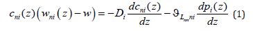
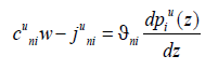
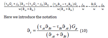
Here z is the spatial variable directed towards the liquid phase, c_ni(z) is the distribution of the concentration of the component n = A, B in the phase i, w_ni(z) is the partial velocity of the component n in the phase i, p(z) is the pressure distribution, and w is the solution velocity. We shall consider that a solution moves in the negative z direction; therefore, w < 0 . i D is the coefficient of component diffusion in the phase i, Lnnni nn ni ϑ = L ϑ , nn L are the phenomenological coefficients, and ni ϑ is the partial specific volume of the component n in the phase i [4]. We shall look for the pressure distribution p^u (z) that gives constant component concentration c^u_ni not taking into account diffusion. In these notations, Fick’s equation (1) takes the form

here we introduce the notation of the component mass flow

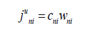
in the phase i. Its solution is

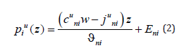
where E_ni is the integration constant. The values of concentrations, mass flows, and integration constants will be found when solving the diffusion problem. On the left side of solution (2), there is the same pressure affecting the particles of different components; however, the forces affecting different components are different. They are determined by the partial volume of the component. As a matter of principle, component mass flows contain partial velocities; therefore, solution (2) can have different values of concentrations in the phases when the mass flow of each component in these phases is equal. The partial velocities in solution (2) are the velocities of component drift caused by the effect of external pressure on the solution. The term with a pressure gradient on the right side of equation (1) describes forces affecting the components. As a result of the effect of these forces, the interface moves. There may be a lot of reasons for the motion of the interface. For example, this is the motion of a temperature gradient through a solution or a phase transition in a metastable solution. Each individual case of a phase transition has its scheme of external phenomena, which lead to the phase transition. For simplicity, we shall assume that a solution moves through a stationary temperature field under the action of a force affecting the external boundary of a solid solution. This scheme is usually applied when using phase transitions to produce materials. When applying a force, pressure arises in a solution. The pressure is transmitted to the interface. The interface shifts and the chemical potential deviates from its equilibrium value at it. As a result it is the deviation of the chemical potential from equilibrium that is the driving force of a phase transition and all the phenomena which accompany the phase transition. It is reasonable to assume that the distribution of pressure caused by an external force in the solution phases has the form of a linear function similar to expression (3). The introduction of external forces affecting multicomponent systems was considered, for example, in [7,8]. In [7], an external force was introduced to the expression of a diffusion flow in the form of a term. In [8], an external force is introduced to the chemical potential in the form of a term; the resulting sum forms a chemical potential with the external force. Both of these approaches are equivalent. We introduce an external force to the problem under consideration, which is caused by the motion of the interface and the drift of solution components in the form of a constant pressure gradient in the solid phase G_p multiplied by the coefficient τ_ni , which is the interaction energy caused by an external field. The introduction of this pressure leads to an additional term in generalized Fick’s equation (1)

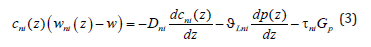
In this notation, it is assumed that in the liquid phase the pressure gradient related to an external force is proportional to G_p , and the coefficients τ_ni take this relationship into account. We make some transformations of Fick’s equation (3) and an equation of the conservation of mass flow

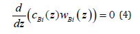
similar to the transformations from [4]. We find the component mass flow c_Bi(z) w_Bi (z) from Fick’s law (3) and substitute it to equation (4). We express a concentration gradient from the obtained equation and substitute it to equation (3). As a result of this transformation, we obtain the following equation:

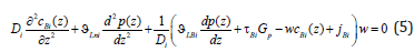
We consider a system of five equations, which consists of generalized Fick’s equation (3) for the component A, equation (5), definition of a mass flow j_Bi=c_Bi (z) w_Bi (z) for the component B, as well as a ratio for concentrations and definition of the solution velocity.

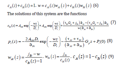
We transform the last term of equation (7).

In contrast to the solution to the diffusion problem from [4,6], a force of external action was included in concentration distribution (7). If 0 p G = , the solutions coincide. This force is assumed to be specified; therefore, the physical meaning of boundary conditions for determining the integration constants of the diffusion problem remains the same. In contrast to [4,6], where the solution velocity was specified, here a solution is assumed to move under the action of an external action force. If a homogeneous solution moved rectilinearly with a constant velocity, this motion would not require an external force, and the solution would move by inertia. In the case of the motion of a solution in which a phase transition occurs, one should consider the effect of thermodynamic forces on solution particles in the interface region where temperature, concentration, or pressure gradients are not zero. According to Le Chatelier’s principle, “When any system at equilibrium is subjected to an external action, processes counteracting this action will take place in the system.” In the case under consideration, this means that when applying a force to the solid phase end, a force balancing the external action force arises in the phase transition region. Under the action of these forces, the solution moves, the temperature at the interface decreases, and kinetic undercooling arises at the interface, which is the driving force of a phase transition, as described in [4,6]. Therefore, all quantities related to the interface motion will depend on the external force G_p .

A question arises that is related to the notation of Fick’s equation in a moving coordinate system. The physical meaning of this transition is as follows. The interface moves through a solution with the constant velocity w. The reason for its motion is a device that shifts the solution and the source of a temperature field through which the solution moves. The shift device and the heat source are assumed to be motionless in a laboratory coordinate system. If the diffusion equation is written in terms of coordinates fixed relative to the solution, its solution will be nonstationary and inconvenient for the analysis. However, some time after the onset of solution motion, on completion of the transition process, the interface will become motionless in a laboratory coordinate system. Concentration, temperature, and pressure distributions will become motionless in a laboratory coordinate system, too. Therefore, the solution to the problem in a laboratory system will be stationary. The transition to a moving coordinate system gives the stationary solution to the problem. It takes into account the velocity of solution motion with respect to a laboratory coordinate system. That is, if a point moving through a solution with the velocity w is taken in the coordinates fixed relative to the solution, this point will be fixed in a laboratory coordinate system. For a formal solution to the problem, it is convenient to assume the interface to be an initial point in a solution. In this case, when a solution moves with the velocity w, in a laboratory coordinate system the interface will have the coordinate z = 0 . However, the motion of the interface with other velocity means that not only a force shifting a solution relative to a laboratory coordinate system but also a temperature field in the vicinity of the interface changed. A change in the temperature field leads to an additional shift of the interface. This can be easily understood if one considers the equilibrium interface as an initial point. In equilibrium, a solution is motionless in a laboratory coordinate system. The force affecting the solution is zero. The coordinate of the interface in a laboratory coordinate system is z = 0 . We switch on the force, the solution moves; after the transition process, the interface moves through the solution with the velocity w. However, its coordinate in a laboratory coordinate system is not z = 0 . The reason is that under the transition to the stationary regime of solution motion, this formal approach loses the processes of the transition regime in which the motion of the solution with a constant velocity and a new pattern of a temperature field is established. During the transition regime, the isotherms are shifted relative to their initial equilibrium position, including the isotherm of the phase transition. This results in the position of a laboratory coordinate system being determined by not only the value of stationary solution velocity but also the shift of the point of the equilibrium phase transition due to a change in the temperature field pattern. Indeed, we denote the coordinate fixed relative to the solution as y. In equilibrium, the interface had the coordinate y = 0. The transition to a system moving with the velocity w is carried out by the change of the variable z = y − wt . It is assumed that in a moving coordinate system the interface continues to be located at the coordinate origin, z = 0 ; i.e., in fixed coordinates the interface has the coordinate y = wt at the time moment t. However, if one considers external effects, the coordinate of the interface will change due to a change in the temperature field in the vicinity of the interface under the transition process to the velocity w . To introduce coordinates in which the interface was located at the coordinate origin, we introduce the distance Δz between the coordinate of phase transition temperature e T , which corresponds to the regime of solution motion with the current value of the velocity w, and the interface. In a linear approximation, this distance will be proportional to the external force, i.e., to the gradient of external pressure in the solid phase

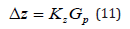
The convenience of this definition is that, if a solution is not affected by an external force, i.e., G_p =0 , the interface has the coordinate of the interface of the equilibrium regime. Of course, this small quantity should not be taken into account when analyzing a particular stationary regime of a phase transition. However, when analyzing a system with an arbitrary velocity of solution motion, the issue of the limiting transition of the system to equilibrium arises. This problem emerged in [4,6]. For its solution, certain conditions were imposed on the kinetics of the addition of liquid solution particles to the solid phase. It will be shown below that the same issue arises in the problem under consideration. The physical issue is that, if one does not take into account ratio (11), within the limit of w→0 the solution to the problem does not describe the equilibrium solution since, as mentioned above, the solution will not coincide with the solution to the problem in the equilibrium regime. This will be obvious when solving the boundary diffusion problem.

In addition to the transition to equilibrium, ratio (11) allows relating the specified pressure gradient in the solid phase G_p to the temperature gradient of a thermal field. If the problem included the description of an external temperature field, at a specified external force the thermal conductivity problem would determine the gradient of the temperature field and the value of kinetic undercooling, i.e., the partial velocities of the components and, therefore, the solution velocity, and the diffusion problem would give concentration distribution. That is, the parameters of the external temperature field and the external force would fully determine concentration and pressure distribution under the stationary phase transition. We specify the value of the temperature gradient G_T at the interface at the known velocity of solution motion. The deviation of the system from equilibrium at the interface is assumed to be small; therefore, we can write the ratio

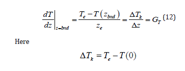
is the kinetic undercooling, and z_bnd is the coordinate of the interface. Note that in a general case, T_e is not the temperature of an equilibrium phase transition but the temperature of the phase transition of a solution at the solution velocity w. Kinetic undercooling determines the velocity of interface motion in terms of the kinetics of the addition of solution particles to a growing phase. In [4,6], the dependence of the velocity of solution motion on kinetic undercooling and the dependence of one component on the kinetic undercooling were introduced. The goal of this formal introduction of the kinetics of the addition of particles to a new phase was the desire to make analytical calculations as simple as possible and state a problem of the conventional scheme of calculation of component distribution under phase transitions. Strictly speaking, this scheme suits only the problems in which the partial velocities of components need not be taken into account. In the problem under consideration, the velocity of component drift plays a crucial role; therefore, expressions for the kinetics of the addition of each component to a new phase are introduced here. We will follow [3] where the partial velocities of solid solution components at the interface are written as

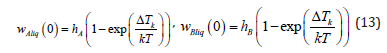
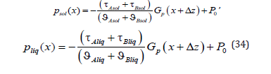
Here h_A and h_B are the constant coefficients, k is the Boltzmann constant, and T is the temperature of the interface, which is assumed to be constant in expressions (13). As a matter of principle, h_A and h_B are determined in terms of the parameters of an equilibrium system. They depend on the distance between the particles of a new phase, the frequency of the addition of the particles to a growing surface, and the structure of the growing surface [3]. Solution velocity is related to the partial velocities by ratio (6). From expressions (11) and (12), it follows that

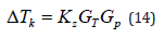
the substitution of (14) to (13) leads to the dependencies of the partial velocities of liquid solution components on the external pressure gradient in the solid phase G_p and the temperature gradient at the phase transition point G_T

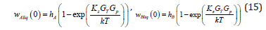
Within the limits of G_p → 0 and G_T →0 , the partial velocities turn to zero, which is fully in accordance with the physical meaning of these quantities. At 0 p G = , no force shifts the solution through the temperature field, and the system is in equilibrium. At 0 T G = , kinetic undercooling is zero; therefore, the temperature of the interface is equal to the equilibrium one, and the interface is motionless. These limits are necessary for the solution to the boundary diffusion problem. To use these limits correctly, we write the solutions in coordinates that take into account the shift of the phase transition point due to a change in temperature field pattern (11). For this to be done, we introduce the x coordinate by changing the variables

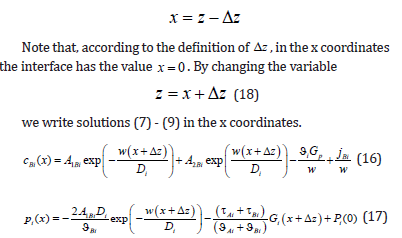
Equations (9) are correct in the x coordinates.

Boundary Conditions for the Problem of Diffusion with an External Effect

Not to complicate the computations, we shall consider a problem with phases in infinite intervals. However, when stating the problem in infinite intervals, formal difficulty arises. The formulation of boundary conditions of the diffusion problem in infinite intervals is known [3]. In the problem under consideration, the value of a pressure gradient at a given point of the solid phase should be additionally specified. At an infinite point, the specification of a pressure gradient under its linear distribution (2) does not have any physical meaning. Therefore, points, at which concentration in a liquid solution and a pressure gradient in a solid solution are specified, will be assumed to be finite but located so far from the diffusion layer that the divergent terms in general solutions to linear equations can be neglected, as was done in the problem in infinite intervals [3]. The problem in infinite intervals describes this physical situation. In this interpretation, we assume the pressure gradient p G in the solid phase to be specified and the phases in the equations to be quite extended. In this case, in solution (16)

We pass to the x coordinate in equations (3) and find expressions for the momentum of the component B from them. The condition of the conservation of component momentum at the interface gives the equation

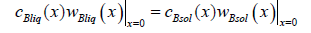
We substitute solutions (16) here and take into account the equality of component mass flows in the phases

After the transformations, the equation of the conservation of the momentum of the component B at the interface takes the form

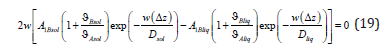
Under condition (18), we obtain

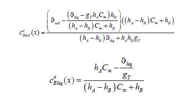
A simple form of the equation of momentum conservation (20) is obtained only in the problem with phases in infinite internals. In the case of finite intervals, all integration constants will be included here. We substitute the values of integration constants (18), (20) to solution (16). When writing concentration distribution in the solid and liquid phases, we obtain

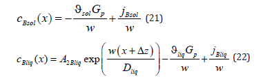
In the solid phase, concentration does not depend on a spatial variable; it depends on solution velocity and a component mass flow. The specification of the value of concentration at an infinite point of a liquid solution does not allow finding the constant 2Bliq A since in the limit of x → ∞ the exponent turns to zero. We get around this difficulty. In equation (22), at x → ∞ we reveal the flow at the point x = 0 , j_Bliq + c_Bliq (0) w_Bliq (0) , and at x = 0 we find 2Bliq A from equation (22). As a result, the distribution of concentration in a liquid solution (22) takes the form

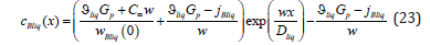
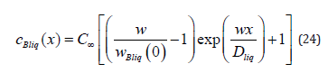
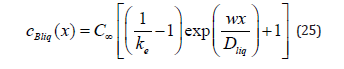
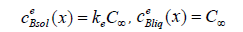
If one removes physical conditions from the statement of the problem under consideration, which distinguish it from the statement of the quasi-equilibrium problem [3], solution (21), (23) passes to the solution to the problem from [3]. In the quasi-equilibrium problem, there is no external driving force; therefore, 0 p G = . The partial velocities of the components far from the diffusion layer in the liquid phase are equal to solution velocity. Therefore, the mass flow of the component B in a solution of the quasi-equilibrium problem is j_Bliq = j_Bsol = C∞ w , and the velocity of the component of a solid solution is w_Bsol(x )= w. Under these two conditions, solution (21) provides the concentration of the solid phase of the quasi-equilibrium problem Ñc_Bliq(x)=∞ . For the liquid phase, the substitution of G_p =0 and the mass flow to (23) gives

According to the definition of a quasi-equilibrium condition, at the interface, the ratio between the boundary concentrations of a solid and liquid solution is equal to the equilibrium segregation coefficient

. The quasi-equilibrium condition and the condition of the constancy of a component mass flow at the interface, c_Bliq (0) w_Bliq (0)= C∞ w , give the ratio of boundary velocities

. The substitution of this ratio to (24) leads to the solution to the quasi-equilibrium problem from [3]

Solution to the diffusion problem (21), (23) allows expressing the concentrations c_Bliq (0) , c_Bsol(0) , the partial velocities w_Asol(0) , w_Bsol (0) at the interface, and the solution velocity w in terms of the partial velocities of the components of a liquid solution at the interface w_Aliq(0) and w_Bliq(0) . For this to be done, we write a system of equations consisting of solution (21) at x = 0

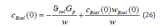
here the expression of a mass flow is revealed. We also write solution (24) at the interface.

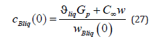
The system of equations also includes the equation of the conservation of a mass flow at the interface

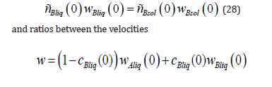
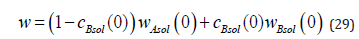
From the system of equations (26) - (29), we find the expressions

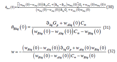
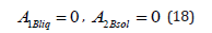
The expression w_Asol (0) is not used in this article. A general solution for pressure distribution (17) includes the integration constants A_1Bi . According to (18) and (20), both of these constants are zero; therefore, pressure distribution in the phases has the form

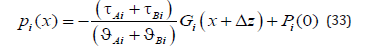
We shall find the integration constants Pi (0) . Strictly speaking, in the problem under consideration, pressure is determined by a force affecting the external boundary of a solid solution. However, for an infinite phase, this force should be infinite. Therefore, only the value of the external pressure gradient p G could be specified. In this case, it is reasonable to specify the ratio of pressure between the phases. In a general case, in the problem under consideration, the deviation of the chemical potential from equilibrium is caused by the deviation of temperature, concentration, and pressure from the equilibrium values [4]. It is known from the experiments that under normal conditions a change in the pressure has little effect on the equilibrium values of the chemical potential, and, therefore, the temperature - concentration equilibrium diagram is used in the calculations. This phase diagram is used in [4] and the present work. That is, a change in the chemical potential due to the pressures of the phases at the interface is not taken into account, and the pressures of the phases at the interface are equal. The equation p_sol (0) = p_liq (0) gives the equality of the integration constants P_sol (0)= P_liq (0)= P0 . Pressure distributions in the phases (33) take the form

Transition of the Solutions to the Equilibrium Regime

When the external disturbance vanishes, G_p → 0, the obtained distributions of concentrations in the phases (21), (23) should transit to the equilibrium regime. A similar problem arose in [4]. The difference is that external action was not introduced in [4]; therefore, the transition of the system to equilibrium meant the limiting transition of the solutions when the partial velocities of the components and solution velocity vanished. In the work under examination, boundary partial velocities of the components (15), i.e., the velocities of the addition of liquid solution particles to a growing phase, depend on the value of the external action p G . If we substitute the partial velocities of the components and the external action being zero to solutions (21), (23), we obtain uncertainty forms of the 0/0 type. For concentration distributions (21), (23) to satisfy the limiting transition to equilibrium, we expand functions (15) into the Maclaurin series with respect to the external pressure gradient G_p , which is assumed to be small, and confine ourselves to a linear approximation.

We reveal mass flows at the interface in solutions (21), (23); then, using expressions of the boundary parameters (30) - (32), we write the solutions with respect to the velocities w_Aliq (0) and w_Bliq (0) . After the transformations, we substitute G_p = 0 to the distribution of concentration in the solid phase. The pressure gradient in solution (21) is reduced. We obtain the expressions for the limits of concentration distributions in the phases (21), (23) at 0

These are the values of the concentrations of the phases in equilibrium; therefore, we obtain two equations

from which we find the kinetic coefficients

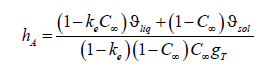
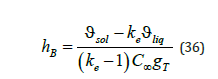
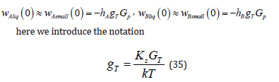
The kinetic coefficients depend on the equilibrium distribution coefficient, the concentration of an initial liquid solution, the coefficients ϑ_sol and ϑé ϑ , which include the partial volumes of the components, and the parameter T g , which, according to (35), depends on the temperature gradient. Taking into account (35), (36), expressions of the partial velocities (15) take the form

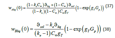
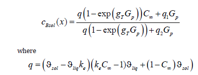
Equations of the kinetics of the addition of liquid solution particles to a new growing phase (37), (38), together with expressions of concentration distribution in the phases (21), (23) and pressure distribution (34), allow calculating the distribution of the concentration and pressure of the stationary regime of a solution phase transition at given parameters. The external pressure gradient G_p and the parameter g_T (35), which depends on the value of the gradient of an external temperature field and the force of the resistance of the interface to external action, are assumed to be specified. The equilibrium segregation coefficient ke , the concentration C∞ at an infinite point of the liquid phase, the partial volumes of solution components ϑni , and the coefficients τ_ni , which take into consideration the relationship between an external force and an external pressure gradient in a solution, are also specified. To demonstrate the properties of the solutions to the problem, we shall limit the domain of variation of some parameters. A solution moves under the action of a pulling force in the direction of negative values of the space axis. Hence, pressure far from the diffusion layer increases in the positive direction; therefore, G_p > 0 . It follows from the derivation of formula (11) that K_z > 0 . We also assume that at the interface a temperature gradient in the liquid phase increases, G_T >0. The partial volumes of solution components ϑ_ni can be both positive and negative. They are included in expressions of the kinetic coefficients ϑ_i (10) in a complicated way. Therefore, their value is limited by the acceptable values of ϑi . The coefficients τni determine the deviation of the partial velocity of a component from solution velocity far from the diffusion layer. This can be seen from equation (3) if the first two terms on the right side are assumed to be zero. They are associated with drift velocity and depend on the mobility of solution components. The derivation of the relationship between τni and mobility is beyond the scope of this article. Since τni do not determine the direction of component motion, it is reasonable to assume that τ_ni >0 . The kinetic coefficients h_A and h_B determine the sign of the boundary partial velocities of liquid solution components (15). According to the statement of the problem, a solution moves in the negative direction; therefore, we confine ourselves to the case of the negative direction of partial velocities. The expressions in parentheses in (15) are negative; therefore, the condition h_n > 0 should be fulfilled. This condition allows limiting the acceptable values of ϑ_i . According to (36), the coefficients h_A and hB are the linear functions of ϑ_i . Therefore, in the (h, ϑ_sol ,ϑ_liq) coordinates, where h denotes hA or hB , these functions are the planes hA(ϑ_sol ,ϑ_liq) and h_B(ϑ_sol ,ϑ_liq). Figure 1 shows the line of intersection of these planes with the plane (ϑ_sol ,ϑ_liq ) at the parameters indicated in Table 1. The letters represent the range where . In the present work, we shall not leave this range of values of i ϑ in numerical calculations. Expressions of the kinetics of the addition of liquid phase particles to a growing interfacial area (37), (38) found from the condition of the transition of a system to equilibrium allow finding some limit relations general for solutions. Distribution of solid phase concentration (21) does not depend on the spatial variable. Its value is equal to the value at the interface (30). The substitution of (37) and (38) to c_Bsol(x)(21) results in the expression

Figure 1:Lines of intersection of the dependencies hA(ϑ_sol ,ϑ_liq) and h_B(ϑ_sol ,ϑ_liq) with the plane (ϑ_sol ,ϑ_liq)

Table 1:Parameter values for the calculation of the plots of Figures 1-3.

We do not write expressions for the constants since they are not used in the present work. In the limit of G_p → ∞ , this expression is the uncertainty form ∞ / ∞ . Under the condition of the problem g_T > 0 , the disclosure of the uncertainty using the known method of numerator and denominator differentiation results in the finite limit

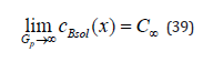
i.e., at a quite large pulling force the concentration of the solid phase is equal to the concentration of an initial liquid solution. Using the same device, we obtain the following limit relations

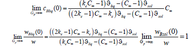
At large values of a pulling force, for the mass flows of the component B in the phases these limits give the simple relations

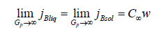
These relations hold for any x.

Segregation of Components by the Interface

We consider the results of the numerical calculations of concentration distribution in the system, the parameters of which are provided in Table 1. The values of the calculation parameters are taken so that the physical relationship between concentration and the external pressure gradient G_p is convenient to interpret in plots. Figure 2 shows concentration dependence on the spatial variable x. At x > 0 , the liquid phase is located; at x < 0 , the solid phase is located. In the figure, the phases are limited by −0.5 < x < 0.5 . These values are far enough from the diffusion layer to illustrate concentration distribution in semi-infinite phases. Without external action, 0 p G = , the phases are in equilibrium. At any G_p , the concentration of the solid phase is constant. When G_p increases from zero, the concentration of the solid phase increases monotonically from the equilibrium value to C∞ . This distinguishes the concentration distribution from the distribution of concentration from [3]. In [3] with semi-infinite phases, at any velocity of solution motion, the concentration of the solid phase is equal to C∞ , i.e., there is a total lack of the segregation of the components by the interface. This contradicts the experiments. To explain this contradiction, it was assumed in [3] that a hydrodynamic flow arises in front of the interface, which specifies an initial concentration of the liquid solution at a distance less than the diffusion layer width. It is quite reasonable that this specification of an initial concentration affects the concentration of the solid phase. This is described in detail in zone melting theory [9]. In this case, the segregation of the components by the interface is explained by a hydrodynamic flow. In [4], pressure is introduced to the diffusion problem. Pressure is introduced by generalized Fick’s law (1). This is not an external force; this is pressure that emerges in a system due to the relationship between the concentration and pressure, which are included in the chemical potential. Outside the diffusion layer, this pressure becomes constant. Hence, outside the diffusion layer, from this pressure there are no forces that affect the solution components. As well as in [3], the segregation of the components by the interface was explained by a hydrodynamic flow. The problem considered above accounts for component segregation by an external force, which results in the emergence of the pressure gradient p G in the system. The force of the pressure gradient affects solution particles throughout the solution, including regions outside the diffusion layer, and results in component drift. This drift determines segregation. This segregation is demonstrated in Figure 2. To explain visually the physical process of segregation, we calculate thermodynamic forces included in generalized Fick’s law (3).

We introduce the notation of forces affecting the component В

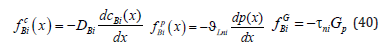
We substitute the distributions of concentrations (21), (23) and pressure (34) in the phases to (40). As a result, we obtain the expressions

Figure 2:Concentration distribution in the vicinity of the interface. 1-Liquid phase,ϑ_liq =0.5 ; 2- solid phase, ϑ_sol = −0.5 .

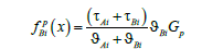
We sum up the forces of each phase

The force of the pressure gradient contains the combination of the parameters τ_ni and ϑ_ni , which is not fully expressed in terms of ϑi ; therefore, we specify them in Table 2 for numerical illustration. Figure 3 depicts the spatial distribution of the forces sum f_Bsol^sum(x) f_Bliq x for four values of the external pressure gradient. According to the calculations, at given parameters the component B in the phases is affected by forces of opposite sign. In the liquid phase, the component B is affected by a force directed in the positive direction. The value of this force decreases monotonically with an increase in the x coordinate. The spatial change in f_Bsol^sum(x) is related to a change in the concentration of the component B in the diffusion layer. In the solid phase, the force f_Bsol^sum(x) is constant and is directed in the negative direction. To find mass flows of the component B in the phases, we solve generalized Fick’s equation (3) for the product of concentration and partial velocity

Table 2:Values of the mass flow, concentration, and partial velocity of the component B for four values of the external pressure gradient.

Figure 3:Dependencies of the force affecting solution particles on the spatial coordinate. 1, 3, 5, 7-the liquid phase; 2, 4, 6, 8-the solid phase; 1, 2,- 0.5 G_p = , 3, 4- 1.0 G_p = ; 5, 6- 2.0 G_p = ; 7, 8- 4.0 G_p = .

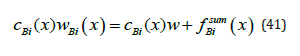
In terms of mass transfer, the quantity c_Bi(x) w_Bi(x) should be considered as the mass flow of a component. On the other hand, as shown in [4], the product of concentration and partial velocity at the interface should also be interpreted as the quantity of momentum. In the physical interpretation of momentum, the product c_Bi(x) w_Bi(x) is the force of inertia of the component B when it moves with a partial velocity. The product of concentration and solution velocity can be interpreted as the force of inertia of the component B when it moves with a solution velocity. We substitute concentration (21), (23) and solution velocity (32) to the right side of equation (41) and find the mass flow of a component for the same values of the external pressure gradient Gp for which the above calculations were performed. The results are provided in Table 2. There, the values of concentration at the point x = −0.5 of the solid phase are also presented. At the point x = 0.5 of the liquid phase, concentration is almost equal to the initial value Ñ 0.15 ∞ = . It is obvious that the mass flow of the component B is the same in both phases. At small values of p G , concentration at the point x = −0.5 differs little from the equilibrium value of the solid phase concentration 0.09 e k C∞ ≈ . With an increase in p G , concentration increases and asymptotically approaches the initial concentration of a liquid solution C∞ . This agrees with calculation of the limit regime (39). This increase in the concentration can be explained by the plots in Figures 2 & 3. According to Figure 3, with an increase in p G a force that “presses” particles of the component B against the interface increases in the liquid phase, and the concentration of the component in front of the interface increases. This leads to an increase in the concentration in the solid phase, and, according to (38), at Gp → ∞ the partial velocity of the component B in the solid phase converges to solution velocity. Hence, in contrast to the problems from [3], an additional degree of freedom arose in the problem under consideration, namely, the motion of solution components outside the diffusion layer under the action of an external force. The velocity of this motion depends on the value of the external force and the mobility of the component in the phase under consideration. The condition of the conservation of a component mass flow in the system is also fulfilled.

Discussion and Conclusion

We shall give a clear physical explanation of the process of component segregation by the interface. For this to be done, we draw attention to three descriptions of the diffusion process under phase transitions. In [3], the equation of convective diffusion is

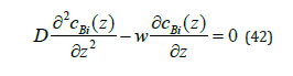
This equation is easy to obtain using Fick’s law

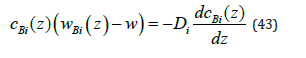
The substitution of the expression of a component mass flow from (43) to equation of a component mass flow (4) gives equation (42). According to (43), in these calculations solution parti cles are affected by one thermodynamic force, namely, diffusion force. When the interface moves, different solubility of components in the phases pushes off the excess of a component to the liquid phase. This leads to the non-uniform distribution of components. A thermodynamic force arises, which strives to return the uniform distribution of components. Formally, the distribution of the component of the problem in infinite intervals in the liquid phase has the form (24); in the solid phase, concentration is constant, ( ) Bsol c z C∞ = . As a matter of principle, in the limit outside the diffusion layer, concentration in the liquid phase is constant. Hence, solution components are not affected by any forces at quite a long distance from the interface. The condition of the conservation of a mass flow at quite a long distance from the interface gives the relationship c_Bliq( ∞) w_Bliq( ∞)= c_Bsol(-∞) w_Bsol(-∞) . At a constant concentration, it follows from Fick’s law (43) that partial velocities are equal to solution velocity, w_Bliq( ∞) w_Bsol( ∞)=w . Therefore, outside the diffusion layer c_Bliq(∞ )=c_Bliq(-∞) . This means the absence of component segregation by the interface. This explanation leads to the conclusion that for segregation to exist, solution particles should be affected by additional forces, which will change their velocities. It is reasonable to assume that this force is a change in pressure.

In [4], pressure is introduced to the system. For this to be done, generalized Fick’s law is used, which is written in the form (3) at p G =0. Similar to the problem from [3], in [4], the solution to the diffusion problem is derived with the specification of the concentration of a liquid solution at the point located at a finite distance from the interface. When introducing pressure, solution particles are affected by not only forces related to diffusion but also forces associated with a change in pressure. However, pressure introduced in [4] results from diffusion. It is included in the chemical potential and does not change at quite a long distance from the diffusion layer. Therefore, in the problem from [4] there is also no component segregation by the interface. This can be easily verified if one passes from the solution in a finite interval obtained in [4] to the solution in infinite intervals. In this case, the concentrations of components in the phases turn out to be equally far from the interface. Only the introduction of an external force (3) leads to the segregation of solution components by the interface. In this case, a term arises in generalized Fick’s law, which describes an external force affecting the particles of the entire solution. All the processes related to interface motion depend on this force. Without the introduction of an external force, the solution velocity was a given value in [3] or was specified by the value of kinetic undercooling [4]. In these works, the solution to the diffusion problem gives constant concentration in the phases far from the interface. Thermodynamic forces included in generalized Fick’s law act only within the diffusion layer; therefore, they do not lead to component segregation. An external force affects solution components both inside and outside the diffusion layer. In the problem in infinite intervals, this results in the partial velocities of a component being different outside the diffusion layer. Therefore, for the condition of the constancy of a component mass flow in the phases to be fulfilled, concentrations also must be different. This is the segregation of components by the interface. We may say that an external force and different mobility of solution particles in the phases lead to segregation. Note that, according to the ratio derived by Einstein [8], the coefficients ni τ are related to component mobility by the expression

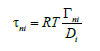
Within the considered problem, this expression is not complete; it does not take into consideration the effect of the partial volume of a component on mobility.

Figure 4:Approximation of the experimental data of Cu distribution in an Al-Cu solution obtained by quenching during solidification [5]. Points - experimental values. Continuous curves - approximation of the experimental data, 1-the liquid phase, solution (23), 2-the solid phase, solution (21).

In conclusion, we explain the result of the experiment from [5], which was provided in the Introduction as an example of component segregation by the interface under phase transitions. In Figure 4, the points approximately give the experimental values of concentration obtained in [5]. The experimentally found values of concentration in Figure 4 are easy to approximate by solution (21), (23). We shall consider the parameters with the values presented in the figure to be specified. According to the figure, an initial concentration of the solution is C∞ ≈ 0.018 . According to the equilibrium phase diagram, at this value of copper concentration in aluminum ke ≈ 0.14 . Dimensional quantities are not introduced in these calculations; however, the values of the diffusion coefficient and the distance from the interface x formally correspond to the experimental values in the SI system of units. The solid lines shown in the figure are the approximation of the experimental values by solution (21), (23) at D_liq = 10⁻⁸ , M_sol =0.5 , M_liq =10 ,Gp = 4.10 ⁻⁷ , and gT =3.10⁶ ⋅ . Solution (21), (23) can correspond to the experimental values only qualitatively since the solution in infinite intervals does not describe concentration distribution in the solid phase. However, this solution accounts for component segregation. It is obvious that to describe concentration distribution in both phases the problem with boundary conditions in finite intervals is necessary. However, the solution to the problem in finite intervals is beyond the scope of this work.

The phase transition of a solution from the liquid phase to the solid one is considered in the present work as an illustration of the mechanism of component segregation by the interface. For practical purposes, condensation, i.e., a phase transition from a gaseous to a liquid state, is no less important. In this case, the densities of phase solutions differ significantly. The condensation of one component can lead to a drop in the pressure of the gas phase in front of the interface. The value of pressure drop, and the extension of the low-pressure region will depend on the velocity of interface motion. It is reasonable to assume that under sufficiently intensive drop formation in the atmosphere, the region of reduced pressure is one of the mechanisms of the formation of atmospheric vortices. The considered problem of diffusion under phase transitions leads to the following conclusion. A correct description of the distribution of solution components under phase transitions requires allowing for an external force that shifts the solution through the phase transition region. The degree of the deviation of solution phases from equilibrium, the kinetics of the addition of solution particles to a new phase, and the interaction between pressure and component diffusion in the phases also need to be taken into consideration.

Data Availability Statement

All data that support the findings of this study are included within the article.

References

1. Guskov AP, Nekrasova LP, Ershov AE, Kogtenkova OA (2013) Decay of the solution in front of the interface under directed crystallization. Materials Science 10: 10-15.
2. Guskov A (2017) Spinodal decomposition of solutions during crystallization. Diffusion Fundamentals 30: 1-9.
3. Jackson KA (2004) Kinetic processes: Crystal growth, diffusion, and phase transitions in materials. Wiley-VCH Verlag GmbH & Co. KGaA, Weinheim, Germany.
4. Guskov A (2021) The condition for the conservation of momentum at the interface under phase transitions of solutions. J Phys Commun 5(055014): 1-12.
5. Chalmers B (1964) Principles of Solidification. Wiley, US.
6. Guskov AP (2021) The effect of new phase growth kinetics and pressure on the distribution of components in phase transitions. Technical Physics Letters 47(6): 540-543.
7. Manning JR (1968) Diffusion kinetics for atoms in crystals. D Van Nostrand Company, Inc, London.
8. Kondepudi D, Prigogine I (2015) Modern thermodynamics: From heat engines to dissipative structures. 2^nd (edn), John Wiley & Sons, Ltd, USA.
9. Pfann WG (1966) Zone melting. John Wiley & Sons, Inc. New York, USA.