
- About Us
- Information
-

The Author ensures that the research has been conducted responsibly and ethically with adherence to all relevant regulations. read more..
- For Authors
- For Reviewer
- Manuscript Guidelines
- Membership
- Publication Ethics
-
- Journals
- Reprints
- e-Books
- Videos
- Policies
- Contact Us
 COVID-19
- Submissions


Full Text
Aspects in Mining & Mineral Science
The Decomposition of a Solution in the Vicinity of a Eutectic Point
Аlex Guskov*
Institute of Solid-State Physics of RAS, Russia
*Corresponding author: Аlex Guskov, Institute of Solid-State Physics of RAS, Chernogolovka Moscow distr, Russia
Submission: September 26, 2022;Published: October 14, 2022

ISSN 2578-0255Volume10 Issue1
Abstract
In the present work, it is shown that being in a non-equilibrium state, a solution can reach an unstable state during the phase transition. In the work, a phase diagram is plotted that demonstrates the boundary of this state, i.e., the boundary of the region of the spinodal decomposition of a solution
Keywords:Decomposition; Solution; Eutectic; Spinodal; Diffusion
Introduction
It is known that for a first-order phase transition, particles should overcome a potential barrier [1]; therefore, the transition occurs when the value of the chemical potential differs from the equilibrium one. When stating crystallization problems, an equilibrium phase diagram is usually assumed to be known, and the dependence of the deviation of the chemical potential from equilibrium is written as the difference between the equilibrium temperature and the interface temperature. It is called kinetic overcooling ΔkT. The velocity of the interface depends on kinetic overcooling, Vs(ΔkT). In the quasi-equilibrium statement [2-4], Δk
Mini Review
The mechanism of the solid phase growth gives the form of the dependence of the structure period on the velocity of the interface motion. This question is considered in detail in [8]. In [10], it was shown experimentally that eutectic composites are formed by the spinodal decomposition of an unstable solution layer in front of the interface. To our knowledge, there exist no works where the possibility of the transition of a solution to an unstable state before its crystallization is considered theoretically and the parameters, a change in which brings thesolution to an unstable state, are found. To explain how a solution can transit to an unstable state we use a simple local configuration model of a solution. In this model, it is assumed [11] that in the crystal lattice of a solution there are positions of two kinds of particles, A and B. The nearest neighbors of the positions of each kind are those of the other kind. In the model, the dependence of mutual potential energy on the distance between the atoms is neglected, and it is assumed to depend on their arrangement only. This rough approximation allows obtaining quite simply the dependence of free energy on component concentration for a multiphase multicomponent system. In this model, an expression for the thermodynamic potential of solutions with the concentration с has the form

here UAА and UВB are the mutual potential energy of two neighboring atoms of one component A or B. The index i denotes the solid phase at i=sol and the liquid phase at i=liq. The quantit
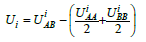
equal to the excess of the mutual potential energy of opposite atoms over the average energy of similar atoms is called mixing energy. Here, UAB is the mutual potential energy of two neighboring atoms of different components, k is the Boltzmann constant, N is the total number of atoms and positions, and lnbi is the logarithmic dependence of entropy on free energy. The transition between the phases itself is the dynamic process of a change in the state of matter under the loss of stability of one phase and the transition of matter to the other phase. When a eutectic periodic structure is formed, two phase transitions occur [10]. A first-order phase transition is the transition of a solution from the liquid to the solid phase, and a second-order phase transition is the spinodal decomposition of a solution. The local configuration model permits showing a change in what physical parameters can bring a solution to an unstable state. To understand what conditions, lead to the unstable state of a solution, we shall use the geometric interpretation of the conditions of phase equilibrium. The liquidus and solidus lines of an equilibrium phase diagram are plotted based on the requirement of the equality of the chemical potentials of solution components at the interface. Geometrically, the procedure is as follows. The dependencies of the thermodynamic potentials of the phases on concentration are plotted for a fixed temperature. A common tangent to two curves of free energy gives the composition of two phases, which are in equilibrium with each other. The concentrations of the components at the tangent points correspond to the abscissas of the liquidus and solidus lines of the equilibrium phase diagram. Between the tangent points, there is the so-called two-phase region. It is clear that the phase transition process occurs in the two-phase region. However, as one can see, the equilibrium diagram does not provide any information on the properties of a solution in the two-phase region. In the two-phase region, the parameters of a solution pass from the values corresponding to the liquid phase to those corresponding to the solid phase. If we plot the dependencies of the thermodynamic potential on concentration with the parameters of a liquid and solid solution and several dependencies with intermediate values of the parameters, we will obtain, for example, the curves shown in Figure 1. The calculations were performed for the following values of the parameters: UAAsol>=UAAliq>=UBBsol>=UBBliq>=1, UABsol>=3.2, bsoul=1.05, bliq, bliq=0.78, k=1, N=1. All the numerical values are conventional. They were selected to obtain an illustrative regular figure. For the sequel, the important thing is that the liquid and solid phases differ in the energy of interaction between solution particles. Here, the upper and lower curves (curves 1 and 6) are the thermodynamic potentials of the solid and liquid phases, respectively. The spinodal decomposition region is in the interval of the temperature dependence of the thermodynamic potential with the convexity upwards. One can see that if the parameters of a solution differ little from those of the solid phase, the solution being in the two-phase region can enter the region of spinodal decomposition. According to the model being used, when a solution transits from the liquid to the solid phase, the concentration of the solution (we assume temperature to be constant) changes due to a change in the potentials of interaction between the particles of solution components and the constant β, which is of no interest in this analysis since it will vanish under differentiation.
Figure 1:Dependence of the thermodynamic potential on the concentration of the solid (1) and (liquid) phases. The parameters UAB andof plotted curves 2, 3, 4, and 5 differ from the difference between values of these parameters of the liquid and solid phases by coefficients of 0.1; 0.25; 0.5; 0.75.

It is clear from the provided plotting that, within the model under consideration, the spinodal region has a boundary on which a variety of system parameters have a certain set of values. If these boundary values of the parameters were known, the boundary of the spinodal region would have to be plotted in the space of these parameters. However, the local configuration model contains a parameter that determines unambiguously the boundary of the spinodal region, i.e., the region where a solution is in an unstable state. This parameter is mixing energy. Indeed, the spinodal regio boundary is determined by zero of the second derivative of the thermodynamic potential with respect to concentration
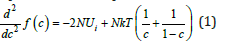
The total number of atoms and positions N is common for both phases. We assume the temperature under a phase transition to be equal to the equilibrium temperature of the phase transition. One can see from this expression that when a solution transits from the liquid to the solid phase, a change in the system parameters is reduced to a change in the mixing energy only. Hence, one can plot an illustrative phase diagram of a solution by including an additional coordinate, mixing energy, to the equilibrium phase diagram. This coordinate, together with temperature and concentration, determines unambiguously the value of expression (1) and, consequently, the boundary of the spinodal region. This diagram is shown in Figure 2. In these coordinates, the liquidus lines b1e1 and f1e1 are in the plane corresponding to the value of mixing energy in the liquid phase. The solidus lines b2a2 and f2d2 are in the plane corresponding to the value of mixing energy in the solid phase. These planes are separated by the space of mixing energy values, as demonstrated in Figure 2. The two-phase region conditionally represents two volumes: that confined by the planes a1e1b1 and a2e2b2, and that confined by the planes e1d1f1 and e2d2f2. In the graph, the boundary of the spinodal decomposition region is plotted. A solution decomposes by spinodal scenario if it enters this region during the phase transition.
Figure 2:A phase diagram with the coordinate of mixing energy values.

Here, a question of principle arises of the sequence of the phase transitions of a solution when it transits from a liquid to a solid state. On the one hand, if a solution enters the spinodal region, it becomes unstable and decomposes into two phases of different compositions. This instability is called instability with respect to diffusion [12]. On the other hand, a solution is in the process of transition from the liquid to the solid phase. As noted above, two phase transitions happen to a solution: a second-order phase transition is the spinodal decomposition of a solution into two phases of different compositions and the phase transition from a liquid to a solid state. This transition occurs when under certain conditions a liquid loses its stability and transits to a crystalline state. This instability is called mechanical instability. As a result, in the problem under consideration, a solution has two types of instability: mechanical instability and instability with respect to diffusion. In this case, an answer to the question of the behavior of a system is given in the monograph by Prigogine [12] where it is shown that for two-component systems mechanical instability is preceded by the emergence of diffusion instability. This means that if in any parameter region a system has mechanical instability and instability with respect to diffusion, first diffusion instability emerges and the spinodal decomposition of a solution proceeds [12].
Conclusion
If during a phase transition, i.e., during a change in the interparticle interaction potentials, the parameters of a nonequilibrium solution enter the spinodal region, it becomes unstable and decomposes into two phases of different compositions. This radically alters our ideas of interfacial mass transfer under phase transitions. So far, it has been assumed that crystallization proceeds from a metastable solution. In this case, a phase transition from the liquid to the solid phase can proceed either on the surface of the solid phase or in the bulk of a metastable solution. If we assume that before crystallization a solution reaches an unstable state, its crystallization will proceed after the spinodal decomposition of the unstable part of the solution. In this case, the composition of the solid phase will depend on the completeness of the spinodal decomposition.
References
- Kondepudi D, Prigogine I (1999) Modern thermodynamics. N Y Wiley, p. 462.
- Jackson KA, Hunt JD (1966) Trans Metal Soc 236: 1129-1142.
- Saito Y (1996) Statistical physics of crystal growth. World Scientific, p. 180.
- Jackson KA (2004) Kinetic Processes. WILEY-VCH, p. 409.
- Mullins WW, Sekerka RF (1964) The Stability of a planar interface during solidification of a dilute binary alloy. Journ Appl Phys 35(2): 444-451.
- Guskov AP (1999) Interphase boundary instabilities at directional crystallization. Bulletin of the Russian Academy of Sciences Physics. Allerton Press, New York, USA, 63(9): 1772-1782.
- Guskov AP (2003) Dependence of the structure period on the interface velocity upon eutectic solidification. Technical Physics 48(5): 569-575.
- Guskov A (2014) On linear analysis of the movement of the interface under directed crystallization. Advances in Chemical Engineering and Science 4(2): 103-119.
- Guskov A (2018) The Formation of two-phase periodic structures. Aspects Min Miner Sci 1(1): 1-6.
- Guskov A, Nekrasova L (2013) Decomposition of solutions in front of the interface induced by directional crystallization. Journal of Crystallization Process and Technology 3(4): 170-174.
- Pines VY (1961) Ozherki on metal physics. Metalshch Kharkov, Ukraine, p. 234.
- Prigogine, R. Defay (1954) Chemical thermodynamics. Longmans Green and CO, New York, USA, p. 509.
© 2022 Аlex Guskov. This is an open access article distributed under the terms of the Creative Commons Attribution License , which permits unrestricted use, distribution, and build upon your work non-commercially.
Editor In Chief


.jpg)


Signup for Newsletter

Quick Links
 Editorial Board Registrations
 Submit your Article
 Refer a Friend
 Advertise With Us
Our Recent Edition

.jpg)


Top Editors


.jpg)


.bmp)
.jpg)
.png)
.jpg)


.jpg)


.png)

.png)


.png)


Financial Support

Sponsors

Latest e-Books

Latest Video

 a Creative Commons Attribution 4.0 International License. Based on a work at www.crimsonpublishers.com.
Best viewed in
a Creative Commons Attribution 4.0 International License. Based on a work at www.crimsonpublishers.com.
Best viewed in