Thermodynamics of the Electrolyte Solutions

Introduction

The coincidence of the formulations of Van Hoff ‘s law for dilute solutions and the equation of state for ideal gases reflects the general statistical regularities that determine the properties of these systems [1]. Moreover, the ideal gas itself is quite similar to a system consisting of particles of solute occupying a volume equal to the volume of the solution [2]. This analogy is also evident in systems with the interaction of components, for example, the Debye-Huckel theory is applicable for both electrolyte solutions and classical plasma in the state of a fully ionized gas. These facts characterizing the observed generality in the behavior of these systems can be taken as a basis for statistical description of the properties of electrolyte solution where the simplest formulations for the ideal gas are used as starting points.

Theory

According to Landau LD et al. [1], the Helmholtz free energy of an ideal gas containing N molecules in volume V can be represent as

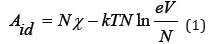
where k is Boltzmann constant, T is temperature, χ is a certain function that depends only on temperature. In a solution that contains interacting components, free energy can be represented as [3]

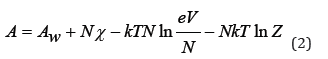
where A_w is free energy of solvent, Z is partition function. Eq.(2) can be generalized for solution containing particles of different grades. So, for a binary electrolyte solution containing N_p cations and N_n anions (N=N_p+N_n), we can write

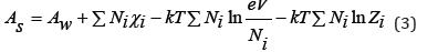
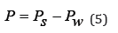
where Zi is the ionic constituent of the partition function. Differentiating Eq.(3) it is possible to determine the pressure in the system

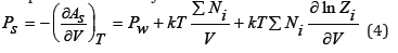
where Pw refers to the pure solvent. Osmotic pressure is defined as

If there are no interactions in the solution and each value Zi=1, the osmotic pressure of the ideal solution can be defined as

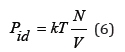
It’s the Van Hoff equation. It bears a close resemblance to the equation of state of an ideal gas and is applicable to ideal solutions regardless of the nature of both the solute and the solvent. Here instead of the pressure of gas there is osmotic pressure, instead of the volume of gas there is volume of solution, instead of the number of particles in the gas there is the number of particles of the dissolved substance.

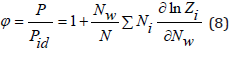
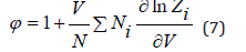where φ is the osmotic coefficient, determined according to Eq. (4) and (6) as

In dilute solutions we can put N<<N_w and V=N_wv_w , where N_w is the number of solvent molecules and v_w is the molecular volume of the solvent. Then Eq.(7) can be represent as [3]

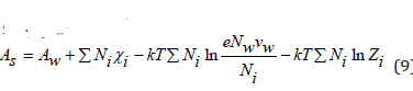
Differentiating Eq.(9), we can determine the chemical potential of solvent in the electrolyte solution

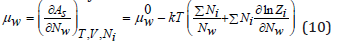
where μw 0 is the chemical potential of a pure solvent. Using Eq.(8), Eq.(10) can be transformed to

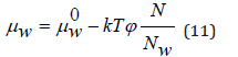
On the other hand, the chemical potential of the solvent can be determined as

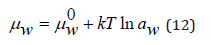
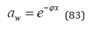
where aw is the solvent activity. Comparing Eq.(11) and Eq.(12), we have

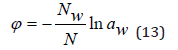
Eq.(13) extends to the entire field of existence of electrolyte solution and is the basis for calculation the osmotic coefficient from experimental data. In aqueous electrolyte solutions, the solvent activity can be defined as and Eq.(13) can be represented in the form

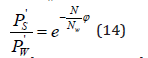
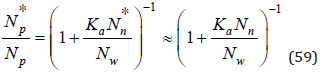
By limiting the exponential expansion to a linear term for dilute solutions, where one can put φ=1, Eq.(14) can be represented as

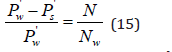
Thus, the relative decrease in vapor pressure during dissolution is equal to the concentration of the solution (Raoul’s law). Eq.(15) contains the relative concentration of the solute x=N/Nw . This value is related to the molality (m) ratio

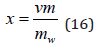
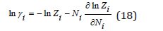
where m_w is the number of moles of the solvent in 1kg (for water m_w=55.51), ν is stoichiometric coefficient (ν = ν_p+ ν_n). Assuming the statistical independence of the ionic constituent of the partition function can determine the chemical potential of each ion

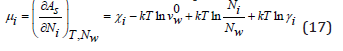
where γi is the ion activity coefficient

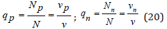
The mean chemical potential can be defined as

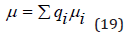
where qi is molar fraction of each ion

Then using Eq.(18) and (19) we have

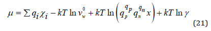
where γ is the mean ionic activity coefficient.

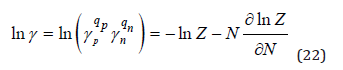
Using Eq.(22) this value can be represented in the equivalent form (since mw is a constant)

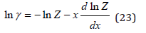
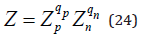
where the partition function of the solution is determined as

The chemical potentials of the solvent and the solute are related by the Gibss-Duhem equation, which, under the condition of constant temperature and pressure, takes the form

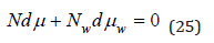
Substituting here the values of chemical potentials, we have

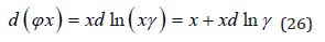
Than using Eq.(23) and integrating Eq.(26) we obtain

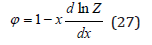
Comparing Eq.(23) and Eq.(27) we also obtain equations

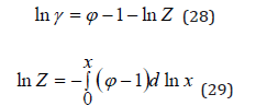
Thus, the partition function of the solution can be determined experimentally. Turning to the theoretical estimation of the partition function of the solution, we assume that the various processes in the solution are independent. Then this value can be represented in form [4]

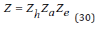
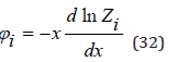
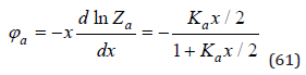
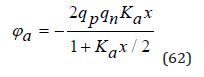
where Zh,Za,Ze are the partition functions corresponding to the processes of hydration, association and electrostatic interaction of ions, respectively. In this case, the osmotic coefficient of the solution can be represented as separate components

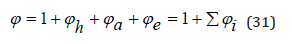
the meaning of which clear from comparing the last equality with Eq.(27) and Eq.(31)

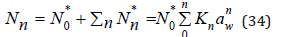
Consider the process of hydration of ions, for example, an anion coordinating n water molecules around itself. The equilibrium constant of this process can be expressed as

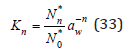
where N0*,Nn* is the number of free and hydrated ions (hydrate complex), respectively. In the formation of various forms of hydrated ions, we can write the equation of material balance

where, according Eq.(33), K0=1.

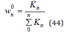
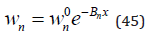
The distribution function for a hydrated ion can be expressed as [3]

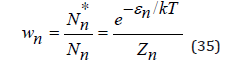
where εn is the difference of the energy between the standard states of the hydrate complex and its constituent components. For a free ion wn makes the form

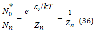
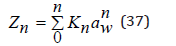
where ε₀=0 is assumed, since this energy level is taken as the reference point. Comparing equations (34) and (36) , the partition function of the ion hydration process can be determined as

To determine the activity coefficient, the partition function mast be normalized. In an infinitely dilute solution, Zn takes value

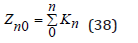
and normalized partition function can be represented as

This normalization condition is obviously not essential for determining the osmotic coefficient, since constant Z_n0 disappears when function ln Z_n* is differentiated.

The mean hydration number an ion is determined as

or using Eq.(35) in the form

where

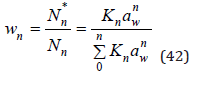
Function ln w_n can be expanded into Taylor series

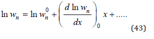
In an infinitely dilute solution a_w=1 and φ=1, then using Eq.(42) we obtain

Limiting to the linear term in the Eq.(43) we have

where according Eq.(13)

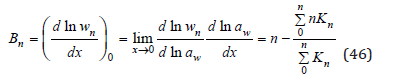
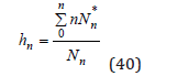
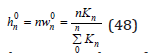
Substitution Eq.(46) into eq.(41) we obtain

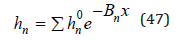
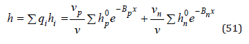
where h_n ⁰ is the hydration number in an infinitely dilute solution

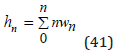
Thus, the mean hydration number of each ion can be represented as the sum of the components containing a various number of water molecules. By combining Eq.(41) and (42), this value can be defined as

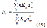
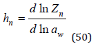
This formula also can be obtained by differentiating Eq.(37)

For another ion, we can write similar equations with a complete replacement of subscripts.

The mean hydration number of the electrolyte can be defined as

and also by an equation similar Eq.(50)

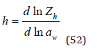
where Z_h is the partition function of the process of hydration of the electrolyte, determined by Eq.(24).

Consider the hydration process in the absence of other interactions in solution. In this case, we can put φh = φ–1. Using Eq.(32), this value can be defined as

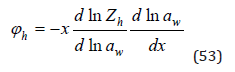
where according Eq.(13)

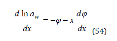
Substitution Eq.(52) and (54) into Eq.(53), we have

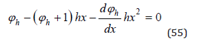
Solving differential Eq.(55), limiting to a quadratic term, imagine as [4]

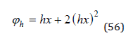
Eq.(56) shows the dependence of the hydration constituent of the osmotic coefficient on the solution concentration.

Turning to the description of the process of ion association in a solution, we restrict ourselves to considering the formation of molecular complexes with ratio of unlike ions 1:1, which is typical for most electrolyte solutions. The equilibrium constant of this process can by determined in the form

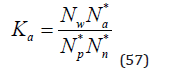
where N_a* ,N_p* , N_n* are the number of associates and free cations and anions, respectively. For each ion species, for example cation, the equation of material balance can be written down

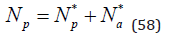
Then from Eq.(57) and (58) we can determine the distribution function of free ions

where, when writing the last equality, the approximation is accepted N_n*≈N_n. Using an equation similar Eq.(36) we have

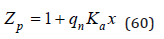
For symmetric I-I and II-II valence electrolytes q_p=q_p and Z_p=Z_n=Z_a , where Z_a is the partition function of the process of ion association. Hence according Eq.(32) we obtain

In general case, for electrolytes of various types, in a good approximation, we can use equation

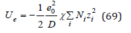
As is known from electrostatics, the energy of the electrical interaction of a system of charged particles can be defined as

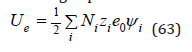
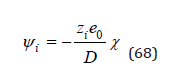
where e0 is the elementary charge numerically equal to the charge of the electron, zi are positive and negative numbers expressing the ion charge in units of elementary charge and ψi is the potential of the electric field acting on the ion from the side of the other charges at the point of location of the selected ion. The Debye- Huckel theory defines the potential of the electric field as [5,6]

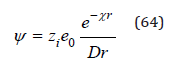
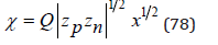
where D=4πε (ε is the dielectric constant of the medium) and χ has a dimension of inverse length

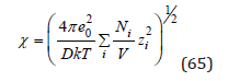
and 1/χ is called the Debye radius. This value can be considered as determining the size of the ionic atmosphere since the field becomes negligible at distances large compared to 1/χ . Based on the principle of additivity of electric fields, the potential ψi can be defined as the Debye potential ψ minus own potential to the selected ion equal (zie0)/Dr it follow

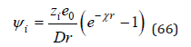
From this expression we can determine the potential at the location of the selected ion using the expansion of the exponential in a Taylor series

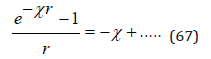
The omitted terms at r=0 turn to zero. Then, the potential ψi can be represented as

Substitution this expression into Eq.(63) we have

Eq.(69) is the basic equation of Debye-Huckel theory, which represents an amendment to the energy due the interaction of ions [6]. However, this correction is found in the variables T,V,N, which does not correspond to the proper variables of the potential Ue. For these variables the thermodynamics potential is the Helmholtz free energy. Therefore, using the well-known thermodynamics equation

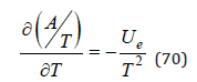
and Eq.(69) one can obtain a relation linking the potentials A_e and U_e for the Coulomb interaction

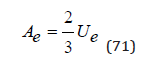
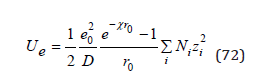
The scope of Eq.(69) is limited to dilute solutions. In this approximation N≪N_w ions can be considered as point charge. However, at high concentrations, the physical size of the ions plays an important role; therefore, the electric field is bounded by a spherical surface at some distance r0 from the center of symmetry where the selected ion is located. In this case, determining ψi for r=r₀ and substituting the result in Eq.(63), the energy of the Coulomb interaction can be determined as [7]

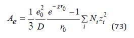
Further, using Eq.(71) we have finally

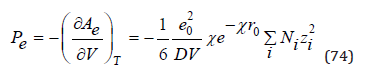
The contribution of the Coulomb interaction to the osmotic pressure of the solution can be determined by differentiating Eq.(73)

and further determine corresponding value

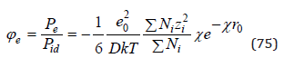
Using definition from which equality 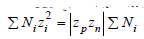follows, Eq.(75) can be represented in a compact form

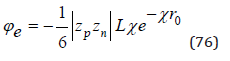
where Similarly, Eq.(65) can be transformed as

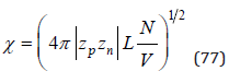
In an infinitely dilute solution assuming as before V=Nwvw , the Eq.(77) can be represented as

where 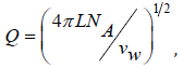NA is Avogadro number, and then present Eq.(76) in a convenient form for calculation

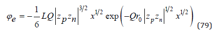
where L 7.156 *10 8 = − cm and Q = 1.735*108 cm-1 for aqueous solution at 298K.

Discussion

From Eq.(76) it follows that the osmotic coefficient in case of Coulomb interaction (φ=1+φe) tends to the ideal value both with dilution of the solution and with increase in its concentration (Figure 1). Such a change in the osmotic coefficient corresponds to the physical meaning of the model under discussion. If the ions were uniformly distributed in the solution independently of each other, then the mean value of the Coulomb interaction energy would vanish, since the solution as a whole is electrical neutral. Therefore, corrections in the thermodynamics values of the solution arise only when the correlation between the positions of various particles is taken into account. Comparing the average distance between particles ~ 1 3 mr c− , where c=N⁄V, and the Debye radius ~ 1 2 Dr c− , which determines the correlation scope, it can be notes that with a decreases in the concentration of the solution (c<1), the ratio rD/ rm increases, so that the correlation captures an increasing number of particles, but the solution becomes ideal because c⤑0. In the opposite case, with an increase in the concentration of the solution (c˃1), the ratio rD/rm decreases and a smaller number of particles appear in the correlation sphere, and despite the increase in the solution concentration, the osmotic pressure tends to the ideal value. To confirm this reasoning, we will give some examples. In dilute solutions, when using approximation 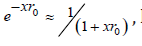Eq.(76) take the form

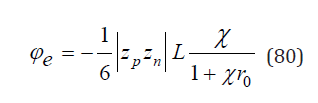
Figure 1: Coulomb component of the osmotic coefficient of aqueous solutions at r0=0.5nm and 298K. 1: I-I valence electrolyte, 2: II-I valence electrolyte.

This formula differs from the result of the Debye-Huckel theory, but fully corresponds to the second virial coefficient in the Pitzer theory [8]. Using Eq.(32), we can determine the partition function corresponding to Coulomb interaction as

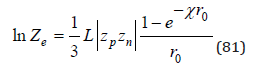
and then obtain the conductivity equation of electrolyte solutions

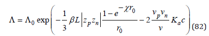
where Λ0 is equivalent electric conductivity in an infinitely dilute solution, c is molarity. This equation described well the experimental data in both dilute and highly concentrated solution, and parameter β is completely consistent with the result of calculation according the Onsager theory [9]. In other cases, when, on the contrary, the Coulomb interaction can be neglected, can be found equation for describing the density of electrolyte solutions [10] and describing thermodynamics characteristics of binary solution of nonelectrolytes [11], and also calculating the separated factor of inorganic substances during crystallization from solutions [12]. However, when calculating the osmotic coefficient of electrolyte solutions, all interaction processes must be taken into account.

Let’s imagine Eq.(13) in a more convenient form for analysis,

from which it is clear that at a given concentration the osmotic coefficient reflects the total interaction of the dissolved substance with the solvent, so the higher its value, the lower the activity of the solvent. Thus, comparing the solvent activity in solutions of various salts at the same concentration, their relative degree of hydration can be estimated, since ions hydration leads to an increase in the osmotic coefficient, and other interaction act in the opposite direction. For example, aqueous solution of alkaline halides can see the growth of the osmotic coefficient in the series of compounds with a common ion (Figure 2): for Cs+ is I< Br< Cl< F, for Rb+ is Br< I< Cl< F , for K+ is Cl< Br< I< F , for Na+ is F< Cl< Br< I , for Li+ is Cl< Br< I. Using a similar construction for cations, all ions can be arranged in order to increase hydration: I≤Cs< Rb< Br< Cl< K< F≤Na< Li. Location in this series of both cations and anions corresponds to a change in the surface density of their charge, so ions of the same species having a smaller size distinguish a greater degree of hydration. From this point of view, the inversion of the osmotic coefficient in a series of anions from F- to I- can be explained when cesium ion is replaced by a sodium ion. Large cesium ion are slightly hydrated; therefore, when replaced with a smaller sodium ion, an increase in the osmotic coefficient is observed. On the contrary, in the series from I- t o F -, when anions are replaced in solutions containing sodium ions, hydration is weakened due to more powerful counteraction from the side of a smaller ion. In the series of alkali metal compounds, when passing from chlorides to hydroxides, hydration is more pronounced, the greater the difference in the sizes of the ions forming this compound (Figure 3). Otherwise, hydration is weakened up to its complete disappearance in solution LiOH, where it is possible to put φ=1+φe (Table 1). Thus, we can formulate a model of competitive hydration, where only one is hydrated, creating a more powerful electric field.

Figure 2: Osmotic coefficients of aqueous solutions of alkali halides at 298K.

Figure 3: Osmotic coefficients of aqueous solutions of hydroxides and chlorides of an alkaline elements at 298K.

Table 1: The parameters for calculating osmotic coefficient of aqueous solutions of electrolytes at 298K.

To calculate the hydrate constituent of the osmotic coefficient we restrict ourselves to a maximum of two form of hydrate complexes and present Eq.(51) in the form

where h₁* and h₂* can belong to one of the ions or to both ions. These values include stoichiometric coefficients, so hydration number of the select ion is determined as h_i⁰=ν/ν_ih_i*. For example, for an aqueous solution of sulfuric acid, the most stable form corresponds to hydration of the proton and the hydration number in infinitely diluted solution is determined as h_p⁰=ν/ν_ph₁*=3/2h₁*≈1. This value corresponds to formula H₃O⁺, and even with solution concentration 76m fourth hydrogen ion is in this form, while the probability of existence of the second form is less than 1/400. This form should also be attributed to the hydrogen ion because of the ion radii r(H₃O⁺)=0,113nm and r(SO₄^2-)=0.24nm [13] it follows that the surface charge density of the ion H₃O⁺ more than twice as high. A similar pattern can be observed in aqueous solution ZnI₂ . (Figure 4) shows the contribution of two hydrated forms, from which it can be seen that at high concentration only the most stable form exist. In the series of zinc halides, there is an increase in hydration during the transition from chloride to zinc iodide due to the weakening of the competitive ability of anions in this series, therefore, the second hydration number in (Table 1) should also be attributed to zinc ion.

Figure 4: Osmotic coefficients of aqueous solutions ZnI2 at 298K. 1: h1*=2.5; B1=1.1; 2: h1*=12.3; B1=15.6; 3: calculated curve and experimental points.

As shown in (Table 1) the above statistical model of binary solution of electrolytes describes well the known experimental data [14,15], with the exception of cadmium halide solutions, where it is possible to form a number of associates, for example, CdI⁺, CdI₂ , CdI₃^-, CdI₄^2- , that requires the use of supplementary parameters. In addition, this model allows us to calculate the osmotic coefficient of dilute solutions based on data from concentrated solution (Table 2), and thus covers the entire area of existence of solution.

Table 2: Osmotic coefficient of dilute electrolyte solutions at 298K.

Conclusion

The statistical model of solution includes the main factors of the deviation of the thermodynamics functions of binary solution of electrolytes from the ideal values–Coulomb interaction, hydration and ion association, and allows us to calculate the osmotic coefficient of solution in the entire area of the existence of solution. This model provides the basis for calculation the separation factor of inorganic substances during crystallization from solution, as well as for calculation the density and conductivity of solutions required for the control of mineral processing technology.

References

1. Landau LD (1995) Lifshits E M Statistical physics, Moscow, Russia.
2. Prigogine I, Kondepudi D (1999) Modern Thermodynamics NY, J Wiley & Sons, USA.
3. Allakhverdov GR (2019) Thermodynamics of solution and separation of elements, Moscow, Russia.
4. Allakhverdov GR (2009) Thermodynamic modeling of aqueous electrolyte solution. Inorganic Materials 45(12): 1532-1536.
5. Debye P, Huckel E (1923) The theory of electrolyte. I, II Phys Z 9: 185-206, 15: 305-325.
6. Debye P (1924) Osmotic equation of state and activity of dilute strong electrolytes. Phys Z 5: 97-107.
7. Allakhverdov GR (2012) Coulomb interaction in electrolyte solutions. Doklady Physics 57(6): 221-223.
8. Pitzer KS (1973) Thermodynamics of Electrolytes I theoretical basis and general equations. J Phys Chem 77(2): 268-277.
9. Allakhverdov GR (2014) The conductivity equation for solutions of strong electrolytes. Doklady Physics 59(5): 206-208.
10. Allakhverdov GR, Zhdanovich OA (2019) Calculation of the density of electrolyte solutions. AMMS 3(3): 418-422.
11. Allakhverdov GR (2013) Thermodynamics of binary solution of nonelectrolytes. Doklady Physics 58(8): 327-329.
12. Allakhverdov GR (2019) Thermodynamics of the separated of inorganic substances during crystallization from electrolyte solution. AMMS 3(2): 382-384.
13. Marcus Y (1983) Ionic radii in aqueous solutions. J Solution Chemistry 12(4): 271-275.
14. Robinson RA, Stokes RH (1959) Electrolyte solutions, London, UK.
15. Mikulin GI (1968) Current issues in the physical chemistry of electrolytes solutions. In: Mikulin GI (Ed.), Khimiya, Leningrad, Russia.