
- About Us
- Information
-

The Author ensures that the research has been conducted responsibly and ethically with adherence to all relevant regulations. read more..
- For Authors
- For Reviewer
- Manuscript Guidelines
- Membership
- Publication Ethics
-
- Journals
- Reprints
- e-Books
- Videos
- Policies
- Contact Us
 COVID-19
- Submissions


Full Text
Aspects in Mining & Mineral Science
Mathematical Modeling of Solid-Liquid Interface Morphology in The Process of Polycrystalline Silicon Directional Solidification
Xuli Zhu1*, Long Xu2 and Hongqiong Wu c3
1 Department of Mechanical and Automation Engineering, Xiamen City University, China
2 Department of Finance, Xiamen City University, China
3 Software Engineering Institute, Xiamen University of Technology, China
*Corresponding author: Xuli Zhu, Department of Mechanical and Automation Engineering, Xiamen City University, Xiamen, China
Submission: October 01, 2018;Published: October 24, 2018

ISSN 2578-0255Volume2 Issue3
Abstract
Two-dimensional mathematical modeling of solid-liquid interface during directional solidification of polycrystalline silicon is established by analytic method. This mathematical model quantitatively reveals the mathematical principle of the solid-liquid interface and can be used to analyze the key parameters affecting the interface morphology. The results of modeling indicate that the interface morphology is related to the boundary temperature distribution of the interface and the heat flux of the crucible sidewall, and the latter is the key factor affecting the interface morphology.
Keywords: Polycrystalline silicon; Directional solidification; Solid-liquid interface; Mathematical modeling
Introduction
Directional solidification is an important process in the physical purification of polycrystalline silicon, the solid-liquid interface morphology in solidification process is directly related to grain size arrangement, grain length and stress distribution [1,2], therefore, the study of the solid-liquid (S-L) interface morphology has important technological value for improving the quality of purification. At present, the theoretical research of S-L interface in directional solidification is often simulated by numerical simulation software [3,4], but the numerical method cannot reveal the intrinsic relation of the parameters, and the analytic method is almost ignored [5,6]. The analytic method, as an exact solution, has an irreplaceable use for the design, process control and experiment of the directional solidification Equipment. we use the two-dimensional mathematical model instead of one-dimensional analysis, it can not only display the interface morphology visually, but also analyze the key parameters, and provide reference for the experiment [7].
Make the following instructions for modeling:
A. The S-L interface occupies only a thin area of the silicon melt, the vertical axis of the melt is set to y, using the symmetry of the crucible. The bottom boundary of thin area W×Δ is set to x axis, so W×Δ is the computational area (Figure 1). Because the area is very thin, the latent heat of solidification released can fill the entire area.
Figure 1:Computational area.

B. The melting temperature of silicon (Tm =14230c) is definite, the discussion of any silicon melt height can represent the whole process of solidification.
Modeling and solving
Because the latent heat is released in solidification process, the
system has an internal thermal source, so the temperature field
satisfies the Poisson Equation, such as Eq. (1)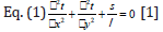
In Eq. (1),
t—Temperature
s— The latent heat
λ —Thermal conductivity of silicon
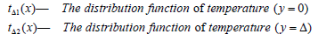
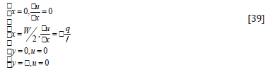
and boundary conditions
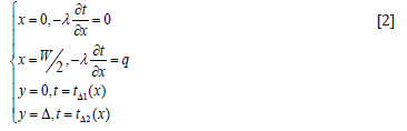
In Eq. (2),
W — The wide of melt
q — Heat flux of crucible side wall
In Eq. (2), x = 0 is symmetrical axis of the crucible, due to the
symmetry of the temperature field, this is Equivalent to a insulation
surface 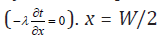 is at the edge of the computational area
(silicon and crucible contact), there may be heat exchange (heat
flux q) with the outside world.
is at the edge of the computational area
(silicon and crucible contact), there may be heat exchange (heat
flux q) with the outside world.
1. When the q > 0, the heat flux is the x axis positive direction, this means that the computational area is losing heat;
2. When q < 0, the heat flux direction is negative along the x axis, this means that the computational area is obtaining heat;
3. When q = 0, there is no heat exchange, the computational area is adiabatic.
Eq. (1) is a Poisson Equation with non-homogeneous boundary conditions, and it is difficult to find the analytic solution directly. The additive (superposition principle) of the differential Equation can be used to convert the Eq. (1) to the sum of Eq. (3) (containing the inner heat source) and Eq. (5), (7) (two Laplace Equations which do not contain the internal thermal source), and then solve.
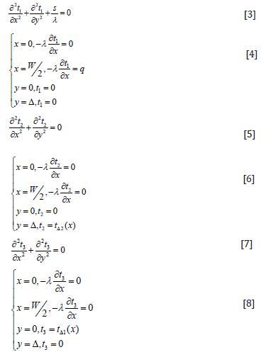
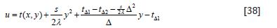
The analytic solution of Eq. (1) can be expressed as

Solve Eq. (3) It is difficult to solve the Poisson Equation directly, and it is generally necessary to convert it to Laplace Equation, and make the following transformation:

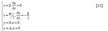
So u satisfies
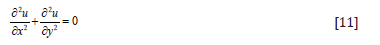
and boundary conditions
Because u is the function of x and y, let

Put Eq. (13) into Eq. (11),
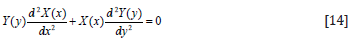
We have
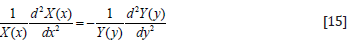
In Eq. (15), only contains x coordinate
  onlycontains y coordinate. To substitute any x, y to make Eq. (15) correct,
and Eq. (15) needs to be Equal to a constant. Let the constant = k2.
onlycontains y coordinate. To substitute any x, y to make Eq. (15) correct,
and Eq. (15) needs to be Equal to a constant. Let the constant = k2.
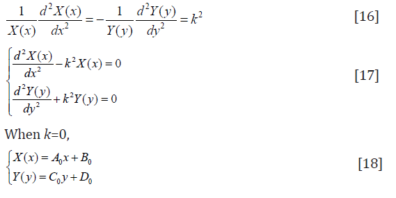
A0, B0, C0, D0 need to be determined. Let
Similarly, A, B, C, D need to be determined. Let

Because trigonometric functions are cyclical, k can be Equal to a series of specific values kn (n=1,2,3…).

Therefore, the general solution of Eq. (11) is

EQUATIONS

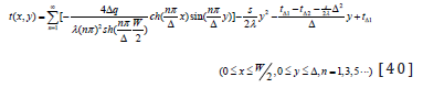
Put Eq. (34), (35), (36) into Eq. (9), the temperature distribution expression t(x,y) in computational area can be obtained.
Discussion
Because the S-L interface is a phase-change surface, the interface is the isothermal surface of 1423 0C. According to Eq. (34- 36), the S-L interface morphology is mainly related to q and tΔ(x), but the analytic solution is very complex, there are many variable parameters, it is difficult to analyze directly. By trial calculation, we know that the q value has the greatest effect on the result. and its value change has a decisive influence on the temperature distribution. Therefore, the heat flux q is the focus of the discussion object.
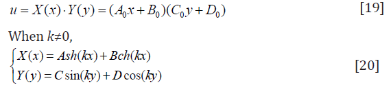
It is assumed that the boundary temperature of the computational area is constant. Eq. (2) can transform to
Solve Eq. (1) on the boundary conditions of Eq. (37). Let
and boundary conditions
Solve Eq. (38) by the separation variable method.
As shown in Eq. (40), the t(x, y) expression is in the form of a triangular series and can draw its function image using commercial mathematical software. Draw images by several different values of the heat flux q. As shown in Figure 2, the computational area W×Δ is properly thickened for looking. The dotted line in Figure 2 represents the S-L interface.
Figure 2:The S-L interfaces in different heat flux.

In Figure 2, when q > 0, the S-L interface shows concave shape, the degree of curvature increases with the increase of q value, and the level S-L interface is at q = 0, which is theoretically ideal. It should be explained that, the interface shape is not simple and evenly curved by Eq. (40), but in general, the concave, convex trend, its curvature radius is non-uniform, not a certain circle of arc.
To obtain the vertical growth of large-size grains, the directional solidification process needs to maintain the S-L interface level, from the above analysis, the side wall heat exchange (heat flux q) has a direct impact for interface morphology, so need to do a good sidewall insulation. However, in fact, there is always a heat exchange because of heater layout, heat dissipation, material performance limitations, control errors and other factors. From the above discussion, the key to determine the level of S-L interface is to make the interface on the same isothermal surface. such as in the directional solidification process, focus on the control of the S-L interface area (W×Δ), temperature control in other melt areas does not need to be too stringent, the S-L interface can still maintain a horizontal shape. This can greatly reduce the difficulty and cost of temperature control.
Conclusion
The following conclusions can be obtained from the above mathematical model:
A. The S-L interface level is Equivalent to the interface in the same isothermal surface, not affected by the temperature distribution of other melt areas.
B. In the thin area (W×Δ), the interface morphology is based on the heat exchange of the crucible sidewall, shows the upper convex, concave and horizontal shape, and the degree of bending depends on the direction and strength of the heat flux q.
When there is no heat exchange (q = 0) on the crucible sidewall, the S-L interface can maintain level when and only when the upper and lower boundary temperature of the area (W×Δ) are constants. This means that it can reduce the temperature control difficulty of the silicon melt.
References
- Ratanaphan S, Yoon Y, Rohrer GS (2014) The five-parameter grain boundary character distribution of polycrystalline silicon. Journal of Materials Science 49(14): 4938-4945.
- Zhu D, Liang M, Huang M, Zhang Z, Huang X (2014) Seed-assisted growth of high-quality multi-crystalline silicon in directional solidification. Journal of Crystal Growth 386(2): 52-56.
- Shur JW, Kang BK, Moon SJ, So WW, Yoon DH (2011) Growth of multicrystalline silicon ingot by improved directional solidification process based on numerical simulation. Solar Energy Materials and Solar Cells 95(12): 3159-3164.
- Lv G, Chen D, Yang X, Ma W, Luo T, et al. (2015) Numerical simulation and experimental verification of vacuum directional solidification process for multi crystalline silicon. Vacuum 116(2): 96-103.
- Hu Y, Hao H, Liu XT (2013) Temperature field analysis of directional solidification of multi-crystalline silicon. Materials Science Forum 750: 96-99.
- Xu M, Zheng L, Zhang H (2014) System design and hot zone optimization of monocrystalline silicon directional solidification furnace for pv application. Journal of Crystal Growth 385(1): 28-33.
- Yi T, Sun SH, Wei D, Xing QZ, Ming JI (2012) Research of solid-liquid interface property during directional solidification process for multicrystalline silicon. Journal of Materials Engineering 2(8): 33-38.
© 2018 Xuli Zhu. This is an open access article distributed under the terms of the Creative Commons Attribution License , which permits unrestricted use, distribution, and build upon your work non-commercially.
Editor In Chief


.jpg)


Signup for Newsletter

Quick Links
 Editorial Board Registrations
 Submit your Article
 Refer a Friend
 Advertise With Us
Our Recent Edition

.jpg)


Top Editors


.jpg)


.bmp)
.jpg)
.png)
.jpg)


.jpg)


.png)

.png)


.png)


Financial Support

Sponsors

Latest e-Books

Latest Video

 a Creative Commons Attribution 4.0 International License. Based on a work at www.crimsonpublishers.com.
Best viewed in
a Creative Commons Attribution 4.0 International License. Based on a work at www.crimsonpublishers.com.
Best viewed in