Integration of Cost Volume Profit Analysis under Uncertainty in Profit Planning: A Current Application

All business activities try to minimize costs to maximize profits. Management determines whether the expected revenues from the expected goods and services will cover the costs that will be necessary for the productive efforts before commencing goods production or service provision. The expected costs may be fixed or variable. In the absence of accurate cost information, managers encounter difficulties in making production, pricing, and other related decisions. Since what is produced has to be sold before revenue can be earned, the company’s profitability depends on (1) costs of production, and (2) the level of sales achieved. Managers use Cost-Volume-Profit (CVP) analysis as a tool to understand the relationships between costs, prices, volume, and profits. However, while managers can control the volume of activity, certainty about costs and prices is elusive under the best of operating conditions. Our main objective in this paper is to demonstrate how C-V-P concepts can be adapted to the overall goal of maximizing expected profits. To this end, various sensitivity analyses based on the stochastic C-V-P model proposed by Hilliard and Leitch [1,2] are conducted. We find that it is better to concentrate on finding and using the expected nominal changes in costs and prices rather than of their dispersion over time. In order to achieve our illustrative goals, we first explain the objectives of C-V-P analysis and review C-V-P analysis under uncertainty. We then describe the stochastic C-V-P analysis model development and perform sensitivity analyses of the stochastic breakeven point. This is followed by illustrative numerical examples that form the basis of our results. We end with a summary of our contributions and the limitations of our work.

Cost Volume Profit analysis helps managers to understand the relationships between cost, volume, price, and profit by focusing on (i) selling price per unit, (ii) variable cost per unit, (iii) total fixed costs, and (iv) sales volume. Jaedicke [3] found that the two typical decision categories used by business management in C-V-P analysis are: (i) decisions related to the required sales volume to attain a target profit level, and (ii) decisions related to the maximum profitable combination of products to produce and market. Management recognizes that planning and control are essential and CVP analysis is one such planning and control tool. A 2003 survey of management accounting practices found C-V-P analysis as one of the most commonly used techniques in accounting Garg et al. [4].

The initial step in C-V-P analysis is finding the breakeven point. The breakeven point occurs when total revenues equal total expenses, thus, profit is zero. At this point, total revenue (TR) minus total variable costs (TVC) and minus total fixed costs (TFC) is zero (TR-TVC-TFC=0). The breakeven point can be determined in units and in dollars once the contribution margin (selling price less variable cost) or contribution margin per unit (CMU) is known, or where the contribution margin ratio (CMR), defined as the contribution margin divided by the selling price, is known. If X is the number of units sold at breakeven point, then at breakeven point, X may be determined as TFC/CMU. Dollar sales at breakeven point may be determined as TFC/CMR. In practice, most companies target a desired net income (after tax income). To achieve this, companies target operating income (TOI) such that when the appropriate tax is taken by the tax authorities, the company will be left with the desired net income. In that case the required units to be sold is determined as [TFC+TOI]/CMU. The dollar sales required to achieve a targeted operating income is determined as [TFC+TOI]/ CMR. Kee [5] proposed that the cost of capital can be incorporated in the C-V-P model. This requires determining the sales quantity needed to break even, as well as the sales quantity required to earn a desired profit or profit margin. Incorporating the cost of capital enables a firm’s manager to evaluate alternative investment and cost structures to enhance a product’s profitability. Kee [5] concluded that “the C-V-P model based on the discounted economic income of products enables managers to compute a product’s breakeven sales quantity, to measure a product’s profitability over the range of its sales, and to determine the rate of change in its profitability” (p. 491). Xi-juan and Jun-ying [6] proposed a stochastic Cost-Volume- Value (CVV) model with economic demand and cost functions. They indicated that the purpose of modern corporate business activities is not profit maximization (C-V-P model), but value maximization because product prices and unit costs are related to volume. They developed a suitable C-V-P model for business value creation and an actual situation under uncertainty. They concluded that the CVV model is more advanced than the traditional C-V-P model, beccause the breakeven point is the volume that takes all the capital costs into account. C-V-P analysis employs a number of important assumptions. These assumptions give rise to some of the limitations of traditional C-V-P analysis. Traditional C-V-P analysis assumes that total cost can be divided into fixed costs and variable costs with respect to the level of output. During the analysis, fixed costs, unit variable cost and the unit selling price of the product remain constant. There is also the assumption that the behavior of total revenues and total costs is linear in relation to output units within the relevant range of activity. In a linear revenue situation, sales mix (the ratio of each product to total sales) and unit prices remain constant. However, selling prices and mixes can change in practice and total revenues may not be linear Edinburg [7]. Furthermore, it is often assumed that units produced are sold, which is not very realistic. Traditional CVP analysis assumes that costs, price, and volume are variables known with certainty. This may not always be the case. The random behavior of such variables creates uncertainty in breakeven analysis Chrysafis [8].

The main limitation of traditional C-V-P analysis is that it does not consider uncertain features of the firm’s operation. Jaedicke [3] presented the first CVP model under uncertainty. They allowed the variables to be random in the basic CVP model. This model is expressed by the following equation Jaedicke [3]; Liao [9]; Magee [10]; Shih [11]:

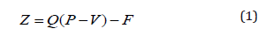
where:

Z: Total Profit

Q: Unit Sales Volume

P: Unit Selling Price

V: Unit Variable Cost

F: Total Fixed Costs

In this equation, the traditional CVP analysis model is appropriate for profit planning under a condition of predictable demand or when the size of demand is unlimited and unsold units can be inventoried and finally sold Shih [11]. There is no adjustment for risk and uncertainty. Jaedicke [3] stated that “the best alternative cannot be chosen without some statement of the firm’s attitude toward risk” (p. 926). Therefore, understanding the amount of risk the firm is willing to accept is crucial to selecting the best alternative. Studies introducing risk or uncertainty into C-V-P analysis have assumed normal distributions of profits Jaedicke [3]; Jarrett [12]; Kim [13]; Johnson [14]; Hilliard [2]. These studies made assumptions that demand and output were equal or unequal. Ismail [15] studied the implications of demand being less or greater than output by considering penalties for inadequate or excess output. They presented the optimization model for the firm by employing the general stochastic model with an uncertain demand and known probability distribution. Other authors analyzed the random behavior of profits by using various distribution methods such as model sampling and curve fitting techniques Liao [9], and lognormal distributiions Hilliard [1].

Research on the relationship between the price and costs using C-V-P analyses under uncertainty have focused on the condition of uncertainty in price and costs, and also established a relationship between price and output volume. These stochastic C-V-P analyses treated price and volume as independent variables. Karnani [16] presented the firm’s risk-return trade off and asserted that the three elements that determine a firm’s competitive strength are (1) cost position, (2) risk-return trade off, and (3) quality of information about uncertain demand and costs. In addition, he indicated that the firm’s position is stronger with lower fixed costs and lower expected variable costs per unit. Also, the lower the value of the firm’s risk and uncertain demand and cost, the stronger it is and the more aggresively it can compete Karnani [16].

Volume of production and sales is one of the most significant causal factors in cost and profit variation. Based on the relationship between price and volume, previous studies have incorporated a demand function in a stochastic C-V-P analysis Kottas and Lau [17,18]; Shao [19]. Chung [20,21] examined the classic C-V-P problem in which volume decisions are based on stochastic information about demand. His results showed that a firm’s output is an uncertain factor and management should be more aggressive in output planning. Said [22] used the cost-volume-profit for both manufacturing and financial service sectors. Wilson [23] provided a case study to explore quality, productivity and cost-volume profit analysis in the contex of solid waste management.

Punlyamoorthy [24] demonstrated how cost-volume-profit analysis established relationships among different elements in the planning of profit, in particular, unit deal value, sales volume, sales mix and settled cost. Souraj [25] explained how the success of an organization is directly related to the effectiveness of its development of innovative products and processes and its implementaion of continous improvement to products or processes. Lulaj [26] showed how much cost-volume-profit analysis is used for planning and making decisions in business. Enyi [27] compared the effectiveness of Weighted-Contribution- Margin (WCM) and Reversed-Contribution-Margin-Ratio (RCMR) in multi product cost-volume-profit analysis applications. Nagar et al. [28] concluded that government economic policy under uncerainity is an important componet of the firm’s information enviroments and manger’s volunatary decisions. Madhani [29] described the importance of customers to whom sales are made, and from whom profits are derived, and underlined the significance of customer focused supply chain strategies to control costs and maximize profits. Oppusunggu [30] emphasized that many small and medium enterprises do not succeed because they do not use the basic profit planning opportunities available to them through CVP analysis. With costs, quantities sold, and prices available to all sizes of companies, she avers that basic CVP analysis is a tool that all businesses should use in practice. Matta [31] presented two optimization models for the strategic formation of supply chain management. While one model used direct costing which treated the fixed production cost as an expense that entirely incurred by the plant producing products, the other model used used fixed absorption costing which included the prorated fixed production cost in the price of outbound product shipments.

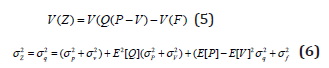
Based on the foregoing, traditional C-V-P analysis has a major limitation; it does not simulate a world of uncertainty. In recognition of this shortcoming, accountants have attempted to use stochastic analysis to provide a better basis for profit planning. “The use of stochastic analysis in a C-V-P analysis model is a great step forward in providing more useful information for profit planning” Liao [9], p. 780). Previous studies on the stochastic C-V-P model have focused on the distribution of profit. Jaedicke [3] proposed a method (hereafter, the JR model) to estimate the distribution of profit in a C-V-P model. They assumed that all the variables including sales volume, unit price, unit variable cost, and fixed costs are normally and independently distributed. The basic equation of their model is Equation 1 above. They considered two sets of assumptions. First, that Q is a normally distributed random variable, while the other variables (P, V, and F) are assumed to be deterministic. Second, total profit (Z) is also normal with mean (μ) and variance (σ) expressed as:

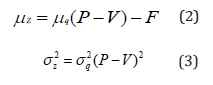
The independence assumption dictated that the mean and variance of profits will be defined by the equation:

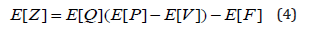
where E[Z]: Expected value of profit. E[Q]: Expected value of sales. E[P]: Expected value of unit selling price. E[V]: Expected value of unit variable cost. E[F]: Expected value of fixed costs. and

Furthermore, the resulting profit is assumed to be normally distributed. The issues with the JR model’s estimation of the distribution of profit in the C-V-P model were identified by Hilliard [1] based on the following two strong assumptions. First, that sales volume, unit price, unit variable cost, and fixed costs are all assumed to be normally distributed. Secondly, that the sales price, variable costs and fixed costs are independent. The problem arising from these assumptions is that due to the normal distribution of parameters in the JR model, the results may tend to be negative when the coefficient of variation is large. Therefore, the JR model has the restriction of small coefficient of variation. In order to overcome the above issues, Hilliard [1] extended the JR model based on the assumption that quantity and contribution margin (P-V) are lognormally distributed random variables. They also assumed that fixed costs (F) are deterministic. Their assumptions lead to a more intuitive distribution for the model’s parameters, allow for dependent relationships (between sales volume, unit price, variable unit cost, and fixed costs), and permit a rigorous derivation of the distribution of the output random variable and profit. In contrast with the JR model, their model does not have the restriction of small coefficient of variation. A follow up article by Hilliard [2] went beyond the approximation of just distribution of profit by developing a general methodology to obtain and utilize the exact distribution of the breakeven point for the stochastic C-V-P model. They concluded from their earlier study that, “if F and C are bivariate lognormal, the ratio of F/C is also lognormal and thus the distribution of the breakeven point is lognormal. The expected value of Log [Qb] is defined in terms of the original input parameters Hilliard [2]:

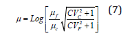
where μf: expected value of fixed costs μc: expected value of contribution (C) σf: standard deviation of fixed costs σc: standard deviation of contribution CVc: coefficient of variation of contribution margin which equals σc/μc CVf: coefficient of variation of fixed costs which is equal to σf/μf The variation of Log [Qb] is expressed by Hilliard [2] as:

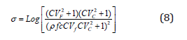
where: ρ fc is the correlation coefficient between fixed costs and contribution margin. Hilliard [2] defined the following statistical relationships between price, variable cost, and fixed costs which are used here to express μ and σ in terms of these parameters.

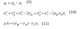
Where

σfv: covariance between fixed cost and variable cost.

σfp: covariance between fixed costs and price.

μp: the expected selling price.

μv: the expected variable cost.

Finally, they expressed the expected breakeven quantity as follows:

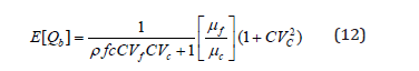
Figure 1 demonstrates the effect of coefficient of variation of the contribution margin on the expected breakeven point Hilliard [2]. In the following section the distribution of breakeven point parameters proposed by Hilliard [2] is examined by applying sensitivity analysis to numerical examples incorporating various selling prices and variable costs. The variations in selling price and variable cost lead to different means and standard deviations, and consequently a different contribution margin (c) is obtained. The effect of the coefficient of variation of the contribution margin on the breakeven point is analyzed.

Figure 1: Effect of the coefficient of variation of the contribution margin on the expected breakeven point, Source: Hilliard JE [2].

Sensitivity analyses of the Hilliard and Leitch model presented above are conducted to study the effect of each parameter on the expected breakeven quantity (E[Qb]). In order to address the sensitivity analyses, a numerical example is presented using Hilliard and Leitch values for the basic parameters which are defined below: μp = $30, σp = 2.40, μv = $20, σv = 1.75, μf = F = $10,000 (deterministic), σf = 0.

Determining the effect of the coefficient of variation of the contribution margin () on the expected breakeven quantity (E[Qb]) is the objective of this illustration and is analyzed implicitly based on the following two scenarios. The first scenario is that all the model’s parameters are constant using the values defined above except the expected selling price and expected variable cost. The second scenario is that all the model’s parameters are constant using the values defined above except the variances of the selling price and the variance of variable cost. The changes in the parameters of the two scenarios lead to different coefficients of variation of the contribution margin. As described above for the first scenario, it is assumed that the expected selling price and variable cost are unknown in the expected breakeven quantity equation. By substituting all other defined parameters in Equation 12 the equation below is obtained:

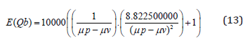
The effect of the E(Q_b) versus μp and μv is demonstrated by a 3D graph produced by MAPLE software in Figure 2. Analysis of the graph demonstrates that as the expected selling price decreases, near to the variable cost, the expected breakeven quantity increases rapidly. In this case, the expected contribution margin (μ_c=μ_p-μ_v) decreases and thus the coefficient of variation of contribution margin (CV_c=σ_c/μ_c) increases. Therefore, it can be said that as CVc increases, E(Q_b) also increases. However, the rate of change in E(Q_b) is intensive when μp is close to μv. In order to better interpret this effect, Figure 3 illustrates the sequence graphs of E(Q_b) as a function of μv based on different μp. It can be said from Figure 3 that when the value of μp is far greater than the value of μv, differences in either μv or μp do not significantly affect the expected breakeven quantity. However, when μp is close to μv, it affects the expected breakeven quantity significantly. The following two examples clarify the above statement.

Figure 2: Expected breakeven quantity vs. expected selling price and variable cost.

Example 1:

The information in Example 1 above shows that as the increases by one unit (Δμ_v=1), the variation of expected breakeven quantity is equal to 2700 units (ΔE(Q_b)=6600-3900=2700).

Example 2:

Figure 3: Effect of μp and μv on expected breakeven quantity.

The information in Example 2 above shows that as the increases by one unit (Δμ_v=1), the variation of expected breakeven quantity is equal to 150units (ΔE(Q_b)=1400-1200=150). We continue to examine the effect of the coefficient of variation of contribution margin (CV_c) on expected breakeven quantity in the second scenario by changing the standard deviation of the selling price (σ_p) and the variable cost (σ_v). By substituting all other defined variables in the base numerical example, the E(Q_b) is expressed as:

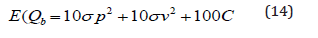
Figure 4: Expected breakeven quantity vs. standard deviations of selling price and variable cost.

The problem is illustrated in Figure 4 by using MAPLE software to produce a 3D graph of E(Q_b) obtained as a function of σp and σv. It can be seen from Figure 4 that as either the standard deviation of the selling price or the variable cost increases, the expected breakeven quantity increases at the same rate. Increases in the standard deviations lead to increases in the coefficient of variation of contribution margin (CVc), and thus expected breakeven quantity E(Q_b) increases. Figure 5 illustrates the sequence graphs of E(Q_b) as a function of σv based on different σp. It shows the rate of changes in E(Q_b) is higher in the higher range of σv and σp. From Figure 5, the variation of expected breakeven quantity, , is higher when the value of either σp or σv is higher. The proof of the above statement is clarified in the following two examples.

Figure 5: Effect of standard deviations of price and variable cost on expected breakeven quantity.

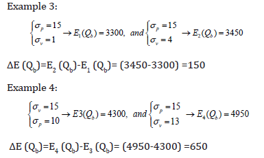
The above results underscore the notion that ΔE(Q_b)in Example 4 is greater than the ΔE(Q_b) in Example 3.

This paper revisited C-V-P analysis and breakeven point with the view to making it better able to capture more of the real uncertain conditions under which businesses operate Beykai [32], Abekah et al. [33], Brockett et al. [34,35]. Traditional C-V-P analysis is used by management as one of the most common accounting planning models in decision-making and profit planning. The traditional model assumes certainty in prices and costs, which leaves out the incorporation of uncertainty. Even where uncertainty is known to exit, inability to properly visualize it has worked against its proper appreciation and therefore limited its fuller incorporation into the planning evaluations. We have therefore used stochastic C-V-P analysis to provide a better basis for profit planning.

We have analyzed a stochastic C-V-P model with a distribution of breakeven quantity Lau [36]. The analyses concentrated on the Hilliard [2] study to obtain the exact distribution of the breakeven quantity for the stochastic C-V-P model by considering lognormal distribution of parameters (F,C,Qb). Furthermore, the effect of the coefficient of variation of the contribution margin () on the expected breakeven point quantity () was determined and analyzed explicitly based on two cases Yunkar [37],Yunkar [38]:

A. Expected breakeven quantity versus expected selling price and expected variable cost.

B. Expected breakeven quantity versus the standard deviation of selling price and the standard deviation of the variable cost.

In the first case all the variables were assumed constant except the expected selling price and expected variable cost. It showed that when expected selling price decreases, the expected breakeven quantity E(Qb) increases in an exponential function. In the second case all the variables were assumed constant except the standard deviations of the selling price and the variable cost. Results showed that as the standard deviation of selling price or variable cost increases, the coefficient of variation of contribution margin (CVc) also increases However, unlike in the case of the nominal selling price and variable cost, the expected breakeven quantity E(Qb) increases at the same rate. The two findings above suggest that emphasis should be placed, as much as possible, on how best to find out expected price and cost changes during the planning horizon. This is because actual prices and costs have much more pronounced impact on operating levels, and hence, ultimate profitability. Reliance on just past price and cost variations will not be very helpful and as they have only proportionate impact of on the potential impact [39].

A major contribution of this work is the use of the Maple Software to operationalize the theoretical models of CVP under uncertainty so that they can be used in practice. Most managers will agree that the certainty and linearity assumptions of the traditional CVP model are sometimes not realistic. However, ways to incorporate uncertainly have largely remained academic and theoretical, thus preventing their practical application. Our graphical demonstrations bring them to life by providing visual demonstrations of the effects of changes in the behavior of CVP variables. With this software’s availability and the possibilities, it presents, we recommended that businesses use CVP analysis extensively, especially in competitive industries and markets. The program will permit the incorporation of more uncertainty into the planning assumptions of any company using it. CVP analysis and planning need not be limited to certainty assumptions. The next step to overcoming a limitation of this study, the non-use of actual company data, is to follow up with by studying and using real life business data in demonstrating the applications of the various examples presented. This is the subject of further an ongoing study. Secondly, the normal or lognormal distribution of the breakeven point presented in this study may not be assertable. The current state of research on this limitation is inadequate and requires further work.

We are grateful for the financial support received, through PDA funds, from the Faculty of Management, University of New Brunswick. We gratefully acknowledge the valuable comments and guidance of SIAM’s reviewers as well as the editorial assistance of our GSTA, Haridas Patel.

1. Hilliard JE, Leitch RA (1975) Cost-volume-profit analysis under uncertainty: A log-normal approach. The Accounting Review 39: 917-926.
2. Hilliard JE, Leitch RA (1979) A stochastic analysis of breakeven points. AIIE Transactions 11(3): 250-253.
3. Jaedicke RK, Robichek AA (1964) Cost-volume-profit analysis under conditions of uncertainty. The Accounting Review 39: 917-926.
4. Garg A, Ghosh D, Hudick J, Nowacki C (2003) Roles and practices in management accounting today. Strategic Finance 85(1): 30-35.
5. Kee R (2007) Cot-volume-profit analysis incorporating the cost of capital. Journal of Managerial Issues 19(4): 478-493.
6. Xi-juan S, Jun-ying F (2007) Stochastic cost-volume-value model with economic demand and cost function. IEEE, pp. 3927-3930.
7. Edinburg LG, Wolcott SK (2005) Cost management: Measuring, monitoring, and motivating performance. John Wiley & Sons, New York, USA.
8. Chrysafis KA, Papadopoulos BK (2009) Cost-volume-profit analysis under uncertainty: A model with fuzzy estimators based on confidence intervals. International Journal of Production Research 47(21): 5977-5999.
9. Liao M (1975) Model sampling: A stochastic cost-volume-profit analysis. The Accounting Review 50(4): 780-790.
10. Magee RP (1975) Cost-volume-profit analysis, uncertainty and capital market equilibrium. Journal of Accounting Research: 257-266.
11. Shih W (1979) A general decision model for cost-volume-profit analysis under uncertainty. The Accounting Review LIV 54(4): 687-706.
12. Jarrett JE (1973) An approach to cost-volume-profit analysis under uncertainty. Decision Sciences 4(3): 405-420.
13. Kim C (1973) A stochastic cost volume profit analysis. Decision Sciences 4(3): 329-342
14. Johnson GL, Simik SS (1974) The use of probability inequalities in multiproduct c-v-p analysis under uncertainty. Journal of Accounting Research 12(1): 67-79.
15. Ismail BE, Louderback JG (1979) Optimizing and satisficing in stochastic cost-volume-profit analysis. Decision Sciences 10(2): 205-217.
16. Karnani A (1982) Stochastic cost-volume-profit analysis in a competitive oligopoly. Decision Sciences 14(2): 187-193.
17. Kottas JF, Lau HS (1978) Stochastic breakeven analysis. Journal of Operational Research Society 29(3): 251-257.
18. Kottas JF, Lau, HS (1979) On handling dependent random variables in risk analysis. Journal of Operation Research 30(8): p.775.
19. Shao, Jun Ying (2007) Stochastic cost-volume model with economic demand cost function.
20. Chung KH (1990) Output decision under demand uncertainty with stochastic production function: A contingent. Management Science 36(11): 1311-1328.
21. Chung KH (1993) Cost-volume-profit analysis under uncertainty when the firm has production flexibility. Journal of Business Finance and Accounting 20(4): 583-591.
22. Said HA (2016) Using different probability distributions for managerial accounting technique: The cost-volume-profit analysis. Journal of Business and Accounting 9(1): 3-4.
23. Wilson KC (2016) Continuous improvement methodologies in public sector of solid west management: A new Brunswick case study. Master of business administration thesis, University of New Brunswick, Fredericton, Canada.
24. Punnlyamoorthy R (2017) Examining cost volume profit and decision tree analysis of a selected company. Journal of Multidisciplinary Research Development 3(9): 224-233.
25. Souraj S (2017) Lean six sigma and innovation: Comparison and relationship. International Journal of Business Excellence 13(4): 479-493.
26. Lulaj E, Iseni E (2018) Role of analysis cvp (cost-volume-profit) as important indicator for planning and making decisions in business environment. European Journal of Economics and Business Studies 4(2): 99-114.
27. Petrik Enyi E (2019) Joint products cvp analysis-time for methodical review. Journal of Economics and Business 2(4): 1288-1297.
28. Nagar V, Schoenfeld J, Wellman L (2019) The effect of economic policy uncertainty on investor information asymmetry and management disclosures. Journal of Accounting and Economics 67(1): 36-57.
29. Pankaj MM (2020) Customer-focused supply chain strategy developing 4Rs framework for enhancing competitive advantages. International Journal of Services and Operations Management 36(4): 505-530.
30. Lis Sintha Q (2020) Importance of break event analysis for the micro, small l and medium enterprises. International Journal of Research-GRANTHAALAYAH 8(6): 212-218.
31. Renato de M (2017) Product costing in strategic formation of research, a supply chain. Annals of Operations Research 272(1-2): 389-427.
32. Beykaei SS (2012) Integration of c-v-p analysis and quality cost in production systems, MBA thesis, University of New Brunswick, Fredericton, Canada.
33. Abekah J, Beykaei SS, Rahim A (2013) Operationalizing cost-volume-profit analysis under uncertainly. Paper presented at the Atlantic Schools of Business Conference, Antigonish, NS, Canada.
34. Brockett PL, Charnes A, Cooper WW, Shin HC (1984) A Chance constrained programming approach to cost-volume-profit analysis. Accounting Review 59(3): 474-487.
35. Brockett PL, Charnes A, Cooper WW, Shin HC (1987) Cost-volume-utility analysis with partial stochastic information. Quarterly Review of Economics and Business 27(3): 70-90.
36. Lau AHL, Lau HL (1987) CVP Analysis with stochastic price-demand functions and shortage-surplus costs. Contemporary Accounting Research 4(1): 194-209.
37. (1914) National Association of cost accountants. The variation of costs with volume. NACA Bulletin 30(16): 1215.
38. Yunker JA (2001) Stochastic cvp analysis with economic demand and cost function. Review of Quantitative Finance and Accounting 17: 127-149.
39. Yunker JA, Yunker PJ (1982) Cost-volume-profit analysis under uncertainty: An integration of economic and accounting concepts. Journal of Economics and Business 34(1): 21-37.