Prediction and Survival Analysis of Head and Neck Cancer in Patients Using Epigenomics Data and Advanced Machine Learning Methods

Cancer is a disease caused by abnormal cell division, causing undesirable cells to form. Normal cells respond to division signals, but cancerous cells undergo genome changes that disrupt normal cell division and death. Malignant cells can pose health risks due to metastasis. Cancer is a multigene, multistep condition originating from an aberrant cell, progressing through natural selection and mutations, ultimately resulting in cancerous cells.

Head and neck cancer

Head and Neck Cancer (HNSCC) is a growing global issue, particularly in Europe, affecting the mouth, lips and tongue. Oropharyngeal and oral cancers are the sixth most prevalent cancers worldwide and early-stage lesions are often not recognized as malignant. Early detection and timely treatment can increase the likelihood of patient survival. HNSCC traditional treatment consists of surgery, radiotherapy and chemotherapy, depending on the tumor and site. However, clinical treatment responses differ greatly among patients with HNSCC, especially in advanced stage disease. HNSCCs are most prevalent in the oral cavity, oropharynx, nasopharynx, hypopharynx and larynx. The prevalence of HNSCC varies between nations and regions and has been linked to excessive alcohol intake, exposure to carcinogens from cigarettes or both. Infection with oncogenic strains of the Human Papillomavirus (HPV), especially HPV-16 and HPV-18, is becoming more associated with the development of oropharyngeal tumors. Effective vaccination campaigns worldwide may help prevent HPV-positive HNSCC, as the two most prevalent oncogenic HPVs are covered by FDA-approved vaccines. Smoking remains the main risk factor for HPV-negative HNSCCs. A study is evaluating the effectiveness of therapeutic dose reduction (of radiation and chemotherapy) in treating HPV-positive HNSCC. HPVpositive HNSCC often has a better prognosis than HPV-negative HNSCC. Most HNSCC patients require multimodality treatments and multidisciplinary care, with the exception of early-stage oral cavity and larynx cancers. The FDA has authorized cetuximab as a radiation sensitizer for recurrent or metastatic HNSCC, but it is less effective than cisplatin as a radio sensitizer in HPV-associated illnesses. Pembrolizumab is licensed as first-line therapy for patients with metastatic cancer and immune checkpoint inhibitors nivolumab and pembrolizumab are approved for treating cisplatinrefractory recurrent or metastatic HNSCC.

Epigenomics and cancer

Epigenomics is the study of gene expression changes influenced by DNA and histone modifications, which can be influenced by environmental and genetic factors. This field has gained significant interest in cancer research, as researchers have discovered that changes in DNA methylation and histone modifications contribute to cancer development by altering gene expression patterns. These changes can serve as biomarkers for early detection and cancer recurrence prediction. Analyzing epigenetic changes in cancer cells allows researchers to identify specific patterns associated with different types of cancer, such as DNA methylation patterns. This information can be used to develop new diagnostic tests and treatments tailored to the specific epigenetic changes associated with each type of cancer. In addition to cancer diagnosis and treatment, epigenomics has the potential to improve cancer prevention. By identifying epigenetic changes associated with increased cancer risk, researchers can develop new strategies for cancer prevention, such as lifestyle modifications or targeted drug therapies. As our understanding of epigenetic mechanisms expands, new advances in cancer research and treatment will benefit patients worldwide.

Background

Head and Neck Squamous Cell Carcinomas (HNSCCs) are the most common cancers in the head and neck region, arising from the mucosal epithelium of the oral cavity, throat and larynx. HPVpositive HNSCCs can be prevented through effective vaccination campaigns, as the two most prevalent oncogenic HPVs are covered by FDA-approved HPV vaccines. Smoking remains the main risk factor for HPV-negative HNSCCs. Advanced-stage HNSCC patients often appear without a clinical history of pre-malignancy, but certain Oral Pre-Malignant Lesions (OPLs) can progress to invasive cancer. Most patients with HNSCC require multimodality techniques and multidisciplinary care, with the exception of early-stage oral cavity cancers, which can be treated with surgery alone. Advances in epigenomic technologies and machine learning algorithms have enabled the analysis of large amounts of data, leading to the development of new tools and techniques to predict the likelihood of head and neck cancer in patients based on their epigenomic profiles. Researchers hope to develop a predictive model that accurately predicts the likelihood of head and neck cancer in individual patients, allowing doctors to provide earlier and more targeted treatments, potentially improving patient outcomes and survival rates. Overall, the use of epigenomics and machine learning in cancer research represents a promising new approach to improving cancer diagnosis, prognosis and treatment. As researchers continue to refine these methods, significant advances in predicting, diagnosing and treating head and neck cancer will be made, ultimately improving patient outcomes and survival rates worldwide.

Head and Neck Squamous Cell Carcinoma (HNSCC), which causes 330,000 deaths and 650,000 new cases annually globally [1,2], is the sixth most common kind of cancer. Nearly all HNSCC patients have Oral Squamous Cell Carcinomas (OSCC) [3]. More than 90% of HNSCC cases are associated with patients with OSCC [4]. South Asian countries including India [5], Bangladesh (Collaboration, 2019) and Pakistan [6] have higher OSCC incidence rates than other parts of the world on average (Collaboration, 2019). Oncogenic viruses such as the Human Papillomavirus (HPV) [7], excessive alcohol use, chewing tobacco usage and cigarette smoking are some of the known risk factors for HNSCC [8]. Additionally, epigenetic regulation, mutation, Copy Number Variation (CNV) and immunological host response have a substantial impact on the development of cancer [9]. Despite recent breakthroughs in cancer detection and treatment, the overall 5-year survival rate for HNSCC is less than 50% due to a lack of suitable diagnostic markers and targeted treatments [10]. In many cancers, including HNSCC, early finding is known to improve survival rates in comparison to late discovery. According to the American Joint Committee on Cancer Stages (TNM), an early-stage primary tumor is one with a diameter of 2-4cm and no lymph node growth or metastases (TNM stage I and II). A tumor is considered advanced (late stage), (https://www. cancer.org/treatment/understanding-yourdiagnosis/staging. html), if it is bigger (>5cm) and has either grown into just nearby lymph nodes (TNM stage III) or has metastasized to other areas of the body (TNM stage IV). Over the past few decades, there has been a lot of new study in HNSCC, but no breakthroughs that are clinically important. Even if certain biomarkers exist (such as HPV +ve and -ve), they don’t have important qualities like high specificity and sensitivity, a low cost or a rapid turnaround. A timely and accurate diagnosis would have several benefits for the patients, such as proper therapy lowering morbidity and enhancing treatment results.

We used HNSC dataset in this study TCGA (http://portal. gdc.cancer.gov) [11]. The data consisted of Radiomics Images of Patients, Clinical Data and Feature Variable Description. Table 1 shows a sample and some of the variables of the Clinical Data of the Patients. The data consisted of 493 patient’s data and 84 columns, which stored the clinical information of the patients. DNA Methylation is an epigenetic modification where a methyl group is added to DNA, influencing gene expression and playing a role in various diseases, including cancer. Histone data comprises information about chemical modifications on histone proteins, influencing gene expression and chromatin structure. Studying histone modifications provides insights into epigenetic regulation, chromatin states, and their roles in biological processes, including development and disease. The human genome is the complete set of genetic material in humans, consisting of protein-coding genes and non-coding regions, enabling the study of genetic variations and their relationship to traits, diseases and human biology. RNA Sequences are transcribed from DNA and provide crucial information about gene expression and regulatory processes. They can be analyzed to identify different RNA types, study alternative splicing, RNA editing and non-coding RNA molecules, enhancing our understanding of gene function and the molecular mechanisms underlying diseases such as cancer. Table 1 shows the Variable Description of all the features present in the Clinical Features data frame. The dataset contains variables such as Patient Identifier, Sex, Age, Date of Birth, Diagnosis of Cancer, Site of Origin and other features related to clinical diagnostic of the patients.

Table 1:OXTR and GAPDH gene primer.

Correlation analysis

Figure 1 shows the correlation analysis among all the variables. Some variables have low positive correlation, and some variables have low negative correlation. The variables that account for “duration” have a perfect correlation of 1 with each other. Radiation treatment dose per fraction is negatively correlated with radiation treatment number of fraction with a value of -0.93. Vital Status is highly negatively correlated to the Overall survival duration, Local control duration, regional control duration, Loco regional control duration, Freedom from distant metastatic duration and Days to last Follow Up with a value of -0.69.

Figure 1:Correlation of analysis.

Survival data exploration

Figure 2 shows the Age of Patients versus the Vital Status (Alive or Dead). It can be confirmed from the grouped histogram that patients who have age more than 55 years have died because of the Cancer. Figure 3 shows the Survival Status of the Patients with the Current Smoking (Yes/No). It can be seen that more patients who are dead who are current smoker as compared to the patients who don’t smoke currently. Figure 4 shows the Cumulative Patients (%) versus Radiation Therapy (RT) Total Dose (Gy) for Alive and Dead patients. RT Total Dose typically refers to the total dose of radiation therapy delivered to a patient during the course of their treatment. The dose is usually measured in units of Gray (Gy) or Centi-Gray (cGy). The total dose is determined by several factors, including the location and size of the tumor, the stage of the cancer and the overall health of the patient. The goal of radiation therapy is to deliver a high enough dose of radiation to kill cancer cells while minimizing damage to healthy tissues. It can be seen that for patient have a higher RT total dose among the age group of 65 to 75 and also chances of survival ae very low around the same. The barchart in Figure 5 shows frequency of Diagnosis status. In medical terminology, “CA BOT” refers to “carcinoma of the base of tongue”, which is a type of cancer that originates from the cells in the base of the tongue. It can be further classified based on the specific type of cells involved and the stage of the cancer. Treatment options may include surgery, radiation therapy, chemotherapy or a combination of these. CA BOT is the most common type of Cancer followed by Tonsils and Super glottic and so on.

Figure 2:Cumulative Patients (%) vs. Age (years).

Figure 3:Survival vs. Current Smoker.

Figure 4:Cumulative Patients (%) vs. RT Total Dose (Gy).

Figure 5:Frequency of each diagnosis.

A. Axial plane: Also known as the transverse plane, this is a horizontal plane that divides the body into upper and lower parts. In CT scans, axial images are taken from the top to the bottom of the body.

B. Coronal plane: This is a vertical plane that divides the body into front and back parts. In CT scans, coronal images are taken from the front to the back of the body.

C. Sagittal plane: This is a vertical plane that divides the body into left and right parts. In CT scans, sagittal images are taken from the side of the body.

By looking at CT scans in different planes, doctors can get a better understanding of the three-dimensional structure of the body and diagnose any medical conditions more accurately. For example, axial images are often used to diagnose issues with the brain, while coronal and sagittal images are often used for imaging the chest, abdomen and pelvis. The images data consisted of images for three different angles for each patient as shown in Figure (6a- 6c). For 182 patients, the image dataset was provided, where 3 images were given for each patient in axial, coronal and sagittal pose. Axial, coronal and sagittal are three terms used to describe different planes of the body in medical imaging, including CT scans [12,13].

Figure 6:(a) Axial image (b) Coronal image (c) Sagittal image.

Numerical feature selection

Correlation based Feature Selection (CFS): Correlationbased Feature Selection (CFS) is a method used in clinical data analysis to identify highly correlated features with a target variable. It calculates the correlation coefficient between each feature and the target variable, indicating the strength and direction of the linear relationship between variables.

Chi-square: The Chi-Square method is a statistical technique used in clinical data analysis to identify significant associations between categorical features and target variables. It compares observed frequencies of each category within a feature with expected frequencies, assuming independence between the feature and target variable. The Chi-Square statistic measures the discrepancy between observed and expected frequencies, with a high Chi-Square value indicating a significant association, and a low Chi-Square value indicating a weaker association.

Mutual information: Mutual Information is a feature selection method that identifies informative features by assessing the information shared between a feature and the target variable [14]. It’s useful in complex data structures and non-linear relationships. Mutual Information is rooted in information theory and measures the knowledge of a feature’s ability to predict the target variable. High Mutual Information values indicate a strong relationship, while low values indicate a weak association. Ranking features based on Mutual Information scores helps select relevant and informative features.

Principal Component Analysis (PCA): Principal Component Analysis (PCA) is a technique that reduces dimensionality and identifies informative features by transforming original features into orthogonal principal components. It aims to capture maximum variance in data by projecting it onto a new coordinate system. Each principal component is a linear combination of original features, ordered by highest variance. Selection of principal components can be based on criteria like contribution to total variance or retaining components explaining a certain percentage of total variance.

Relief-F: Relief-F is an iterative feature selection method for high-dimensional, noisy data, estimating feature quality based on difference in nearest neighbors, with features with significant differences being more informative for classification. Recursive feature elimination: Recursive Feature Elimination (RFE) is an iterative process used to select the most important features from a dataset by removing less relevant ones. It helps machine learning models achieve desired performance levels by training on the full set of features and removing the least important ones.

Image-based feature extraction

Canny edge: Canny Edge is a popular feature extraction method used in computer vision and image processing for edge detection. It is named after its inventor John Canny and is known for its effectiveness in detecting edges in images while reducing noise sensitivity. The edges detected by Canny Edge can be valuable features for image-based classification tasks.

Sobel edges: Sobel Edges is a gradient-based feature extraction method for edge detection in images, named after inventor Irwin Sobel. It uses convolutional operations and filters to compute gradient magnitude and direction, highlighting horizontal and vertical edges. The gradient magnitude represents edge strength, while the direction provides edge orientation. This technique simplifies detecting and extracting important features related to edges.

Linear Binary Pattern (LBP): Linear Binary Pattern (LBP) is a texture-based feature extraction method widely used in computer vision. It captures local texture patterns by comparing the intensity values of pixels in an image neighborhood. LBP can effectively represent texture information and has been utilized in numerous image classification and object recognition applications.

Deep learning and classification

Transfer learning is one of the advantages of Deep Learning, a developing topic of study. For instance, in image classification, Transfer Learning uses characteristics that have been homed in one domain and applied to another through feature extraction and fine-tuning. Convolutional Neural Network (CNN) models have been employed with remarkable success on various comparable or different datasets, large or small, and were trained on ImageNet’s million photos with 1000 categories [15,16]. Small datasets can benefit from these pre-trained networks because only the higher layers of these pre-trained networks need to be trained on the new datasets. This is because the lower layers of these pre-trained networks already contain many generic features like edge and color blob detectors. Since 1995, studies on transfer learning have gained increasing amounts of attention under various names, including “learning to learn,” “lifelong learning,” “knowledge transfer,” “inductive transfer,” “multi-task learning,” “knowledge consolidation,” “context-sensitive learning,” “knowledge-based inductive bias,” “meta learning,” and “incremental/cumulative learning.

Figure 7:Explained variances for PCA.

Clinical features-based modelling: After conducting the Exploratory Data Analysis and visualization, we processed the data before modelling to create and process all the variables that are contained in the dataset. Initially, we drop the features that are not present at the time of early diagnosis from the dataset. After dropping these variables, we created Dummy Variables for Categorical features and for the numerical variables, we scaled variables from values -1 to 1. After pre-processing the dataset, we applied Principal Component Analysis (PCA) on the pre-processed dataset and selected 10 principal components as shown in Figure 7. After transforming the features to PCA variables, we split the dataset into train and test set. The training data had 55 observations and test data had 14 observations. We built three models for building classifier with clinical data only and described below.

Fully connected network of back propagation neural network (FCN/BP): The first layer of the FCN/BP consisted of a choice of many nodes, which were 128 with Dropout choices of 0.1 and Activation choices of Relu functions. Similarly, second layer consisted of choice of many nodes, which were 32 with Dropout choices of 0.1 and Activation choices of Relu functions and followed third layer with choice of many nodes, which were 32 with Dropout choices of 0.2 and Activation choices of Relu functions. The last layer was the output layer with two nodes and sigmoid activation. The final model architecture is shown below in Figure 8.

Figure 8:FCN/BP architecture.

Long short-term memory (LSTM): The first layer of the LSTM consisted of a choice of many nodes which were 64 with Dropout choice 0.05 and Activation of tanh functions. Similarly, second layer consisted of choice of many nodes, which were 64 with Dropout choice 0.3 and Activation of tanh function followed by third fully connected layer with choice of many nodes which were 288 with Dropout 0.1 and Activation choice of Relu functions. The last layer was the output layer with two nodes and sigmoid activation. The final model architecture is shown in Figure 9.

Figure 9:LSTM architecture.

Convolutional neural network (CNN): The first layer of the CNN consisted of a choice of many nodes which were 128 with Dropout choice 0.2. Similarly, the second CNN layer consisted of choice of many nodes, which were 32 with Dropout choice 0.2 followed by third fully, connected layer with choice of many nodes, which were 128 with Dropout 0.2 and Activation choice of tanh function. The last layer was the output layer with two nodes and sigmoid activation. The final model architecture is in Figure 10 below.

Figure 10:CNN architecture.

Image feature-based modelling

We explored the performance of various models, such as VGG16, ResNet50, DenseNet, ResNet101 and Xception. Initially, we implemented these models without applying any feature selection methods. This involved training the models on the complete set of available features. To further investigate the impact of feature selection, we incorporated three popular techniques: Canny Edge, Sobel Edges, Linear Binary Pattern. These methods aimed to improve the models’ performance. The image-based feature selection methods are applied to the dataset. In methods, first it reads the image and converts it to grayscale. Then calculates the image. And after that appends the calculated image to features list. After processing all the images, the features list is converted to a 3-dimensional array with RGB channels. This allows for visualization purposes and compatibility with certain downstream models that require RGB input. By utilizing the feature selection methods, we were able to extract local texture patterns from the grayscale images. These patterns can then be used as features for further classification tasks using VGG16, ResNet50, DenseNet, ResNet101, Xception model.

Image feature and clinical feature bases modelling: Data was loaded from each patient folder using glob API, and the file location was stored in a data frame. We converted the images into the NumPy array and stored them into pandas’ data frame against identifiers to merge the features with the clinical features. Below output shows the dimensions of the Images which shows 69 number of observations or total number of patients, images of 128x128 pixels with 3 channels (RGB). The PCA applied Clinical features have 69 observations or total number of patients with 10 principal components features.

a) Shape of Images Features: (69, 128, 128, 3).

b) Shape of PCA applied Clinical Features: (69, 10).

c) Shape of Labels: (69,) which consists of labels which are 0 or 1.

The shape of labels is a 1-dimensional array, which consists of labels as either 0s or 1s. Thereafter, the data was split into training and test sets. The training set consisted of 55 number of observations and the test set consisted of 14 number of observations.

A. Training Images Features Shape: (55, 128, 128, 3)

B. Testing Images Features Shape: (14, 128, 128, 3)

C. Training Clinical Features Shape: (55, 10)

D. Testing Clinical Features Shape: (14, 10)

E. Training Labels Shape: (55)

F. Testing Labels Shape: (14)

G. After pre-processing and preparing the data, we performed modelling.

VGG16-FCN: The results below show the VGG16 model experiments. We conducted 100 experiments for each model. The following is the flow diagram of VGG16 -FCN Model. The chosen parameters are highlighted in Figure 11 below.

Figure 11:VGG16-FCN architecture.

DenseNet121-FCN: The results below show the DenseNet121 model experiments. We conducted 100 experiments for each model. The following is the flow diagram of DenseNet121 -FCN Model. The chosen parameters are highlighted in Figure 12 below.

Figure 12:DenseNet121-FCN architecture.

ResNet50-FCN: The results below show the ResNet50 model experiments. We conducted 100 experiments for each model. The following is the flow diagram of ResNet50 -FCN Model. The chosen parameters are highlighted in Figure 13 below.

Figure 13:ResNet50-FCN architecture.

Xception-FCN: The results below show the Xception model experiments. We conducted 100 experiments for each model. The following Figure 14 is the flow diagram of Xception -FCN Model.

Figure 14:ResNet50-FCN architecture.

ResNet101-FCN: The results below show the ResNet101 model experiments. We conducted 100 experiments for each model. The following Figure 15 is the flow diagram of ResNet101 -FCN Model.

Figure 15:ResNet50-FCN architecture.

Survival analysis by kaplan meire method

A collection of statistical operations for data analysis using time to an event happens as the outcome variable of interest is known as a survival analysis. The occurrences might include things like death, illness, client attrition and recuperation. Simply said, it is used to determine how long a population under investigation will live. It is also known as “Time to Event” analysis since its objective is to determine how long it will take a certain person or group of people to experience a particular event of interest.

The following formula may be used to calculate the likelihood of surviving at any given time:

S(t) = exp(−H(t))

Where S(t) is the survival probability at time t and H(t) is the cumulative hazard function up to time t.

The Kaplan-Meier estimator is a non-parametric method of estimating and visualizing the survival probability as a function of time. It is also known as the product-limit estimator. Given that it is the most straightforward method and calls for the fewest assumptions, it is frequently the initial step in the survival analysis process. We use the following assumptions in order to do the analysis using the Kaplan-Meier method:

a) The survival probability of all observations is the same, regardless of when they joined the research.

b) The event of interest is unambiguous and occurs at a clearly defined time.

c) The chances of censored observations surviving are no different from those of followed observations.

We are hardly aware of the genuine survival function in practical situations. In order to approximate the real survival function from the gathered data, we use the Kaplan-Meier estimator. The estimate is given by the following equation and is defined as the percentage of observations that survived for a specific period under identical conditions:

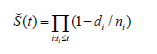
Where:

A. Š(t)is the estimated survival probability at time t

B. Π is the product symbol, which indicates the multiplication of each individual probability

C. t_iis a time when at least one event happened,

D. d_i is the number of events (e.g. deaths) that occurred before time t_i,

E. n_i represents the number of individuals known to have survived up to time t_i, (they have not yet had the death event or have been censored). To put it differently, the number of observations at risk at time t_i.

Hardware details

The Nvidia GTX 1050 GPU was used in a project to train Deep Learning networks 8X faster than an i7 Intel CPU running at 3.5GHz. GPUs are ideal for parallel processing, as they have a large number of cores that can work together simultaneously to perform complex calculations. CPUs have fewer cores and are better suited for sequential processing tasks. GPUs can parallelize and accelerate large numbers of matrix multiplications, allowing for faster execution time for deep learning tasks. The GPU has 640 CUDA cores and a memory bandwidth of 112GB/s, allowing for efficient data transfer between the GPU and CPU.

Each possible strategy for classification ought to be examined by employing a separate set of assessment criteria. Therefore, we utilized a 10-fold cross-validation by randomly splitting the samples inside a dataset into 10 folds of break even with an estimate. After calculating ten execution degree values and comparing them to 10-folds, the Standard Deviation (std) of these values is used to determine the framework’s execution. The same method is repeated for each dataset that is being analyzed. The models were evaluated using the accuracy, precision, recall and F1-score [17].

Modelling results

Tumor classification with clinical features only (without feature selection methods): Table 2 shows the results of tumor classification using clinical features without feature selection methods. Three models were used: FCN, LSTM, and CNN. The LSTM model achieved a higher accuracy score of 93.0%, while the FCN and CNN models had 86.0% and 0.898, respectively. The precision score was 0.94, with the LSTM model having the highest score of 0.94. The recall score was 0.93, with the LSTM model having the highest score of 0.86. The F1 score was also highest for the LSTM model, with 0.93. Overall, the LSTM model performed best in terms of accuracy, precision, recall and F1 score, possibly due to its ability to capture temporal dependencies in the data. However, the results were obtained without feature selection methods, which may affect the performance of the models.

Table 2:Results of tumor classification with clinical features only (without feature selection methods).

Tumor classification with image features (without feature selection methods): Table 3 shows the results of tumor classification using image features without feature selection methods. Four metrics are used to evaluate the models: accuracy score, precision score, recall score and F1 score. VGG16 has the highest accuracy score of 79.0%, followed by DenseNet121 with a lower score of 56.99% and a precision score of 0.571. ResNet50 has an accuracy score of 86.0%, while Xception has a lower score of 56.99% and a precision score of 0.571. ResNet101 has the highest accuracy score of 93.0%, precision score of 0.94, recall score of 0.93 and F1 score of 0.93. Overall, ResNet101 outperforms DenseNet121 and Xception, with high precision and recall scores.

Table 3:Results of tumor classification with image features (without feature selection methods).

Tumor classification with clinical features and image features (without feature selection methods): Table 4 shows the results of tumor classification using clinical and image features without feature selection methods. The table lists various models, including VGG16-FCN, DenseNet121-FCN, ResNet50-FCN, Xception-FCN and ResNet101-FCN. The performance of each model is evaluated using four metrics: accuracy score, precision score, recall score and F1 score. The VGG16-FCN model achieved 79.0% accuracy, while DenseNet121-FCN, ResNet50-FCN, Xception-FCN and ResNet101-FCN achieved 56.99% accuracy, 0.898, 0.86 and 0.86, respectively. The ResNet101-FCN model achieved the highest accuracy score of 93.0%, while DenseNet121-FCN and Xception- FCN performed the worst.

Table 4:Results of tumor classification with clinical features and image features (without feature selection methods).

Tumor prediction-clinical features only (all feature selection methods): Table 5 shows results of tumor prediction using clinical features using various feature selection methods [18]. Results showed that FCN, LSTM, and CNN models with CFS, Chi-Squared, LSTM with RFE, Select-kBest and Select from Model achieved the highest accuracy scores of 91.54% and 0.915, respectively. CNN models with PCA method had the lowest accuracy scores of 64.9% and the lowest precision, recall and F1 scores of 0.770, 0.654 and 0.707, respectively. The best feature selection method varied across different models, with dark green representing the highest score and orange representing the lowest.

Table 5:Results of tumor prediction-clinical features only (all feature selection methods).

Table 6:Results of tumor prediction-image features only (all feature selection methods).

Tumor prediction-image features only (all feature selection methods): Table 6 is showing the performance of four pre-trained deep learning models (VGG16, DenseNet, ResNet50 and Xception) for tumor prediction using different image feature extraction methods and feature selection methods [18]. The Sobel method, which detects edges in images, performed well for ResNet50 and VGG16 models, while the Canny method did not perform well for ResNet50 and Xception models. The HOG method, which captures edge orientation distribution, performed well for ResNet50 and Xception models, but not for DenseNet and ResNet101 models. The LBP method, which encodes local texture information, performed well for Xception but not for VGG16 and ResNet101 models. Overall, the choice of deep learning model, feature extraction method and feature selection significantly impact the performance of a tumor prediction model using image features.

Tumor prediction-clinical features + image features (all feature selection methods): Table 7 shows the results of tumor prediction models using various Feature Selection (FS) methods [18], including VGG16-FCN, DenseNet-FCN, ResNet50-FCN, Xception-FCN and ResNet101-FCN. The models were trained using four different FS methods: Sobel, Canny, Histogram of Oriented Gradients (HOG) and Local Binary Patterns (LBP). They were trained using two clinical data FS methods: Correlation-Based Feature Selection (CFS) and Chi-Square. The results showed that the choice of FS method significantly impacted the performance of the models. ResNet50-FCN performed well with Canny and Chi Square, while DenseNet-FCN had the lowest performance with HOG and Chi Square. Some models consistently performed well across different FS methods, while others were more sensitive to the choice of FS method. CFS and Chi Square performed similarly across most models and FS methods, but CFS performed better with HOG and LBP, while Chi Square performed better with Canny and Sobel. The study’s results can guide future FS methods selection for future tumor prediction models.

Table 7:Results of tumor prediction-clinical features + image features (all feature selection methods).

Survival analysis

The Kaplan-Meier test is a statistical method used in medical research to estimate and compare survival rates of patients with various conditions, including Head and Neck Squamous Cell Carcinoma (HNSCC). This powerful tool helps identify groups with higher risk of death and lower survival chances, enabling more targeted and personalized treatment options. It can be used to compare survival rates based on factors like age, gender, smoking status, tumor size and location, enabling researchers to develop more targeted and effective treatment plans. Additionally, the Kaplan-Meier test evaluates the effectiveness of different treatments, such as surgery, radiation therapy, or chemotherapy, helping clinicians identify the most effective treatments and improve patient outcomes.

Gender versus vital status: Figure 16 shows the survival rate of the Patients w.r.t. Gender, it can be confirmed that Male Patients are more prone to death as compared to female patients.

Figure 16:Survival analysis of gender versus vital status.

Smoking status versus vital status: Figure 17 presents the Kaplan-Meier analysis comparing smoking status with vital status. This analysis examines the survival probabilities of individuals based on their smoking status. The x-axis represents the time in the study, while the y-axis represents the estimated survival probability. Overall, the Kaplan-Meier test is a valuable tool for HNSCC research, allowing researchers to gain a better understanding of the disease and develop more effective treatments to improve patient outcomes.

Figure 17:Kaplan meier analysis of smoking status versus vital status.

This research focuses on predicting head and neck cancer in patients using epigenomics and survival analysis, machine learning and deep learning methods. The best model was ResNet50 with Sobel feature selection method for image data and Relief F-based feature selection for clinical features, with a test accuracy of 97.9%. The ResNet101 model performed best with Histogram of Gradients feature selection method for image data and mutual informationbased feature selection for clinical features, with a test accuracy of 96.1%. The Kaplan-Meier test in Survival Analysis has provided valuable insights into the survival outcomes of patients with Head and Neck Squamous Cell Carcinoma (HNSCC). Factors like gender, smoking status, tumor laterality, cancer sub-site of origin, HPV status and T-category were analyzed to assess their impact on vital status and survival probabilities. Results showed that certain factors were associated with higher death risks and lower survival chances. The role of the anti-aging gene Sirtuin 1 may be critical to the higher death rates and lower survival chances. Sirtuin 1 may be important to predict head and neck cancer in patients using epigenomics and survival analysis, machine learning, and deep learning methods [19-21]. Current smokers had a higher death probability compared to former or non-smokers, while patients with cancer from soft palate, base of tongue and tonsil sub-sites showed increased vulnerability to mortality. Overall, the Kaplan- Meier test has contributed valuable insights to understanding HNSCC and has the potential to enhance patient management and outcomes in the future. In future, we can work on other cancer cell diagnosis such as breast cancer, lung cancer, bone cancer, blood cancer, oral cancer etc. The accuracy level and methodology of our research and analysis results can help us to work more on such datasets. We can make more profound choices on how to merge the datasets, apply more hybrid techniques, collect and build capacity to harness more data for more patients and come up with a predictive model, which is highly accurate as our model and can be used in real time predictions.

Conceptualization-Kalpdrum Passi; Data curation-Vikaskumar Chaudhary; Formal analysis-Vikaskumar Chaudhary; Investigation- Vikaskumar Chaudhary; Methodology-Kalpdrum Passi, Vikaskumar Chaudhary and Chakresh Jain; Project administration-Kalpdrum Passi and Chakresh Jain; Resources-Kalpdrum Passi; Software- Vikaskumar Chaudhary; Supervision-Kalpdrum Passi and Chakresh Jain; Validation-Vikaskumar Chaudhary; Visualization-Vikaskumar Chaudhary; Writing-original draft-Vikaskumar Chaudhary; Writing-review & editing-Kalpdrum Passi and Chakresh Jain.

1. Rizzo PB, Zorzi M, Mistro AD, Mosto MC, Tirelli G, et al. (2018) The evolution of the epidemiological landscape of head and neck cancer in Italy: Is there evidence for an increase in the incidence of potentially HPV-related carcinomas? Plos One 13(2): e0192621.
2. Kapoor A, Kumar A (2019) Head-and-neck dermatofibrosarcoma protuberans: Scooping out data even in dearth of evidence. Cancer Research Statistics and Treatment 2(2): 256.
3. Deshpande AM, Wong DT (2008) Molecular mechanisms of head and neck cancer. Expert Review of Anticancer Therapy 8(5): 799-809.
4. Vigneswaran N, Williams MD (2014) Epidemiologic trends in head and neck cancer and aids in diagnosis. Oral and Maxillofacial Surgery Clinics of North America 26(2): 123-141.
5. Poddar A, Aranha R, Royam MM, Gothandam KM, Nachimuthu R, et al. (2019) Incidence, prevalence and mortality associated with head and neck cancer in India: Protocol for a systematic review. Indian Journal of Cancer 56(2): 101-106.
6. Akhtar A, Hussain I, Talha M, Shakeel M, Faisal M, et al. (2016) Prevalence and diagnostic of head and neck cancer in Pakistan. Pakistan Journal of Pharmaceutical Sciences 29(5): 1839-1846.
7. Marur S, D’Souza G, Westra WH, Forastiere AA (2010) HPV-associated head and neck cancer: A virus-related cancer epidemic. The Lancet Oncology 11(8): 781-789.
8. Stenson KM, Brockstein BE, Ross ME (2016) Epidemiology and risk factors for head and neck cancer. UpToDate.
9. Leemans CR, Snijders PJ, Brakenhoff RH (2018) The molecular landscape of head and neck cancer. Nature Reviews Cancer 18(5): 269-282.
10. Wiegand S, Zimmermann A, Wilhelm T, Werner JA (2015) Survival after distant metastasis in head and neck cancer. Anticancer Research 35(10): 5499-5502.
11. Grossberg A, Mohamed A, Elhalawani H, Bennett W, Smith K, et al. (2018) Imaging and clinical data archive for head and neck squamous cell carcinoma patients treated with radiotherapy. Scientific Data 5: 180173.
12. Ojala T, Pietikäinen M, Mäenpää T (2002) Multiresolution gray-scale and rotation invariant texture classification with local binary patterns. IEEE Transactions on Pattern Analysis and Machine Intelligence 24(7): 971-987.
13. https://image-net.org/.
14. Zhang L, Li H, Liang Y, Li X (2020) A review of feature selection methods based on mutual information. Entropy 22(10): 1075.
15. Guyon I, Elisseeff A (2003) An introduction to variable and feature selection. Journal of Machine Learning Research 3: 1157-1182.
16. Pan SJ, Yang Q (2010) A survey on transfer learning. knowledge and data engineering. IEEE Transactions on Knowledge and Data Engineering 22(10): 1345-1359.
17. Huang J, Ling CX (2005) Using AUC and accuracy in evaluating learning algorithms. IEEE Transactions on Knowledge and Data Engineering 17(3): 299-310.
18. Brownlee J (2014) Feature selection with the scikit-learn library. Machine Learning Mastery.
19. Martins IJ (2016) Anti-aging genes improve appetite regulation and reverse cell senescence and apoptosis in global populations. Advances in Aging Research 5: 9-26.
20. Martins IJ (2017) Single gene inactivation with implications to diabetes and multiple organ dysfunction syndrome. Journal of Clinical Epigenetics 3(3): 24.
21. Martins IJ (2017) Nutrition therapy regulates caffeine metabolism with relevance to NAFLD and induction of type 3 diabetes. Journal of Diabetes Metabolic Disorders 4: 019.