Detection and Classification of Brain Tumors by Analyzing Images from MRI Using the Support Vector Machines (SVM) Algorithm

Introduction

Generally, brain tumors can be classified in two primary and secondary classes [1].

Primary brain tumors

Tumors located in brain tissue are known as primary brain tumors. The type of tissue in which they arise classifies the primary brain tumors. Gliomas, which rapidly grows and spreads into the adjacent glial tissues, is the most common primary brain tumor.

Secondary brain tumors

Secondary brain tumors are actually caused by cancer in other parts of the body and are completely different from primary brain tumors. The concept of spreading cancer cells in the body is called metastasis. When cancer cells move to the brain tissue from other parts of the body and spread there, the cancer is called with the same name from that organ of the body. For example, if one person is diagnosed with lung cancer and these cancer cells spread throughout the brain, the brain cancer is called metastatic lung cancer. This is because the cancer cells in the brain resemble the ones in the lung. There are different kinds of treatments for secondary brain tumors which depend on the factors below [2-4]:

a. Location of the first cancer cells

b. Extent of the spread

c. Patient’s age

d. Patient’s overall health

e. Patient’s respond to previous treatments

The progress of MRI as a clinical asset has been extraordinary, out striping the development rate of other imaging methods. This speed of growth is a testimony to its clinical significance. The medical imaging specialists and their clinical colleagues have not been slow to grasp the advantages of an investigation which produces clear anatomical display in any plane, with no radiation risk to the patient, and with a tissue discrimination unrivalled by any other imaging technique. This process has accelerated, and new clinical applications are being defined constantly. Any new imaging method is followed by an educational need; in the case of MRI, dynamics of technology and applications create our greatest challenges for continuing education [5]. The basics of MRI can be explained in two ways; classically and via quantum. The nucleus contains nucleons which are subdivided into protons and neutrons; protons are positively charged, neutrons have no net charge, and electrons are negatively charged. The atomic number is the sum of the protons in the nucleus, and the mass number is the sum of the protons and neutrons in the nucleus. The atom is electrically stable if the number of negatively charged electrons orbiting the nucleus equals the number of positively charged protons in the nucleus. The atoms that are electrically unstable due to a deficit, or an excess number of electrons, are called ions.

Given the clinical information about the brain tumor from the MRI images, we would be able to reduce the negative effects of the tumor to a great extent. For a more effective treatment, we can use more information such as size and the number of tumors [6]. MATLAB is a multi-model numerical calculation surrounding and a dedicated programming language created by mathematicians. This program can be used for manipulating and changing matrix, plotting and showing the functions and various data, and implementing different algorithms. This program gives the ability of user interfaces and interfaces with other programs even those which are written in a different coding language. In this research, we will elicit the number, size, and position of the tumors by processing MRI images using MATLAB software under certain algorithms.

Material and Methods

MATLAB is an information analysis and incarnation tool with many advantages:

a. It can be used easily in matrix operations;

b. It has excellent graphic options;

c. It has a powerful programming language;

d. It has preinstalled programs for different particular tasks.

These original programs are called toolboxes. One of these toolboxes is the image processing toolbox which is crucially important for our project. In this research we focus only on those capabilities of MATLAB that concern image analysis, function description, and the required commands and techniques. The function of the program is that it takes various parameters in and produces an output: for example, a matrix, a string, a graph, or a figure. There are many toolboxes in MATLAB which make it a software with multiple functions. A new custom function can also be added to the program any time. In machine learning, support vector machines (SVMs, also support vector networks) are supervised learning models with associated learning algorithms that analyze data used for classification and regression analysis [7]. When a set of training examples is given to SVMs, these examples are marked due to the categories they belong to. Then, SVMs training algorithm builds a model that defines new examples for each relevant category, which make a non-probabilistic binary linear classifier. Although there are some methods like Platt scaling that uses SVMs in a probabilistic classification setting (Figure 1).

Figure 1:Schematic for transform processing.

To describe an SVM model, we can say that it is like a map whose examples are shown like points in a space. Therefore, the examples of each category are completely separated from those of other categories. SVM can perform a non-linear classification by the “kernel trick”; which map the inputs in to high-dimensional feature spaces. When the data is not marked, controlled learning is not possible. So, an uncontrolled learning approach is necessary. This way the datum that does not belong to either of the categories is found. This new data can be useful in future approaches and it improves the support vector machines, when the datum is not labeled or when only some of the data are labeled as a processing for a classification pass. Therefore, the new group can be designed. This way a linear classification has happened [8]. On the other hand, a support machine builds up a hyper-plane or a group of hyper-planes in an infinite dimensional space. These hyper planes can be used for classification, regression and outlier’s detection [9]. Generally, the larger the margin, the lower the generalization error of the classifier. Therefore, when the hyper plane has the largest distance to the nearest training data point of any class, a desirable separation is achieved.

We are given a training dataset of {\displaystyle n}nn points of the form where the {\displaystyle y_{i}} y_i either 1 or -1, each indicating the class to which the point {\displaystyle {\vec {x}}_{i}} belongs. Each {\displaystyle {\vec {x}}_{i}} is a ρ dimensional real vector. We want to find the “maximum margin hyper plane” that divides the group of points{\displaystyle {\vec {x}}_{i}} for which {\displaystyle y_{i}=1} y_i = 1 from the group of points for which{\displaystyle y_{i}=-1} y_i = −1 , which is defined so that the distance between the hyperplane and the nearest point {\displaystyle {\vec {x}}_{i}} {\displaystyle {\vec {x}}_{i}}from either group is maximized. Any hyper plane can be written as the set of points {\displaystyle {\vec {x}}}satisfying.

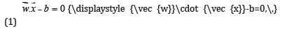
Where {\displaystyle {\vec {w}}}is the (not necessarily normalized) normal vector to the hyper plane. This is much like Hesse normal form, except that{\displaystyle {\vec {w}}} is not necessarily a unit vector. The parameter{\displaystyle {\tfrac {b}{\|{\vec {w}}\|}}} determines the offset of the hyperplane from the origin along the normal vector{\displaystyle {\vec {w}}} [10]; (Figure 2).

Figure 2:Maximum-margin hyper plane and margins for an SVM trained with samples from two classes. Samples on the margin are called the support vectors.

Hard margin

When the training data is linearly separable and we choose two parallel hyper planes (which separates the two classes of data), the space between them would be as large as possible. The space between two parallel hyper planes is called the “margin”. When the hyper plane lies halfway between two parallel hyper planes, the maximum margin hyper plane would occur. These hyper planes could be described as equations below:

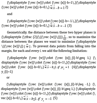
These constraints show that each data point must lie on the correct side of the margin; this can be rewritten as:

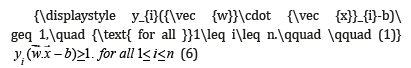
Then we place all these data together to get the optimization problem:

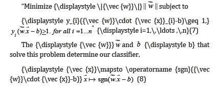
The consequence of the aforementioned geometric description is that the max-margin hyper plane is completely determined by those which lie nearest to it. These {\displaystyle {\vec{x}}_{i}} are called support vectors [11]. Where the parameter λ {\ displaystyle \lambda }determines the tradeoff between increasing the margin-size and ensuring that the {\displaystyle {\vec{x}}_{i}} lie on the correct side of the margin. Thus, for sufficiently small values of{\displaystyle \lambda } λ , the soft-margin SVM will behave identically to the hard-margin SVM if the input data are linearly classifiable, but will still learn if a classification rule is viable or not [12]. Synthetic digit images are used for training. Each of the training images has a digit surrounded by other digits which stimulates how digits are normally seen together. Using synthetic images is appropriate and without having to collect the samples manually, it enables you to create a variety of training samples. For testing, scans of handwritten digits are used to validate how well the classifier performs on data which is different from the training data. This is not the most indicative data set, but there is sufficient data to train and test a classifier and show the possibility of the approach.

Training Set = image Data store (synthetic Dir, ‘Include Subfolders’, true, ‘Label Source’, ‘folder names’);

Test Set = image Data store (handwritten Dir, ‘Include Subfolders’, true, ‘Label Source’, ‘folder names’);

Use count Each Label to tabulate the number of images associated with each label. In the example below, the training set consists of 101 images for each of the 10 digits and the test set consists of 12 images for every digit (Figure 3); (Table 1 & 2).

Table 1:

Table 2:

Figure 3:Training and test images.

Ans=10x2 table

Show a few of the training and test images

Figure: Subplot (2,3,1);

Im show (training Set. Files {102});

Subplot (2,3, 2);

Im show (training Set. Files {304});

Subplot (2,3, 3);

Im show (training Set. Files {809});

Subplot (2,3, 4);

Im show (test Set. Files {13});

Subplot (2,3, 5);

Im show (test Set. Files {37});

Subplot (2,3, 6);

Im show (test Set. Files {97});

The first step to train and tests a classifier (a pre-processing step) is applied to remove noise artifacts which were affected during collecting the image samples.

% Show pre-processing results

Ex Test I mage = read image (test Set, 37);

Processed Image = im binarize (rgb2gray (ex-Test Image));

Figure: Subplot (1,2,1)

Im show (ex-Test Image)

Subplot (1,2,2)

Im show (processed Image) (Figure 4).

Figure 4:A pre-processing step is applied.

Using HOG features

The HOG feature vectors which are elicited from the training images are used to train the classifier. Therefore, it is important to make sure the HOG feature vector encodes the right amount of information about the object. The extract HOG Features function gives a visualization output that can be helpful to clarify what is meant by the “right amount of information”. By changing the HOG cell size parameters and visualizing the result, you can see how affective that could be on the amount of shape information encoded in the feature vector.

img = read image (training Set, 206);

%Extract HOG features and HOG visualization

[hog_2x2, vis2x2] = extract HOG Features (img,’ CellSize’, [2 2]);

[hog_4x4, vis4x4] = extract HOG Features (img, ‘CellSize’, [4 4]);

[hog_8x8, vis8x8] = extract HOG Features (img,’ CellSize’, [8 8]);

%Show the original image

Figure: Subplot (2,3,1:3); im show(img);

%Visualize the HOG features

Subplot (2,3,4);

Plot (vis2x2);

Title ({‘CellSize = [2 2]’; [‘Length=’num2str (length(hog_2x2))]}); (Figure 5)

Figure 5:Using HOG features.

Subplot (2,3,5);

Plot (vis4x4);

Title ({‘Cell Size = [4 4]’; [‘Length=’num2str(length(hog_4x4))]});

Subplot (2,3,6);

Plot (vis8x8);

Title ({‘Cell Size = [8 8]’; [‘Length=’num2str(length(hog_8x8))]});

This research indicates that if we give a cell size of [8 8] to the program, it doesn’t encode much shape information; but when we use cell size of [2 2] as the input, it encodes much shape information. In the meantime, it increases the HOG feature to a noticeable extent. The cell size of [4 4] would be the perfect compromise, because it would encode enough spatial information for a digit shape to be identified as well as limiting the number of dimensions in the HOG feature vector, which accelerates the process of training. Practically, the HOG parameters should be put to test repeatedly to identify the finest parameter settings.

Cell Size = [4 4];

Hog Feature Size = length (hog_4x4);

Using this algorithm and the mentioned method, we process the MRI image, and the output will be a clear image of the tumors and the number and size of the tumors.

Diagnosis of brain tumor through MRI image analysis in MATLAB

General description of the project: Many methods of tumor diagnosis have been studied and tested in the previous researches, but the lack of a combined method consisted of multiple processes has always been felt. In this project, we managed to reduce the time factor leaving the quality unchanged using SVM Training Algorithm. The function is: quick analysis of the MRI image, increasing the image quality, and then removing the noise from the picture. The image then will be processed using the SVM algorithm to diagnose and classify the tumor.

SVM: Using the SVM machines presented by Vapnik is one of the globally widespread methods of machine training and template diagnosis. SVM makes its predictions by using a lineal combination of Kernel function on a series of training data known as the supporting vectors. SVM training is different from other methods in respect that it always finds the overall minimum. The qualities of an SVM are to a great extent relative to its Kernel selection. SVM training leads to a (QP) second degree programming which can face many problems in the numerical solution methods in big portions of examples. Therefore, to simplify the solution method, there are multiple methods introduced which can be put to practice. In this project, we first discuss machine training, classifying and introducing the discussed SVM, and then the equation related to training in SVM. Generally, machine training can be done in two, supervised and non-supervised, methods many use supervised machine training methods. These methods consist of a group of input vectors like nX={X} and output vectors such as nT={t}. the purpose is for the machine to be able to predict the t given new x inputs. For that, two separate conditions can be considered: regression, in which the variable is continuous, and classification, in which the t belongs to a discrete collection. Many of the machine learning cases are subset to the second group and the aim of the machine training is for the machine to be able to make a proper classification. As an example, consider that the aim is to design and train a machine which can detect and tell apart a face image and a non-face image. This system practically does nothing but classification. If we consider an n-dimensional x vector for each input datum (in this case the input image), the machine must be able to classify the x vectors which are seen as points in the n-dimensional space. The machine is required to be trained and tested for new amounts of inputs in the training process. The training of the machine cane be considered in a mathematic form i→yix. As a matter of fact the machine is defined by a series of possible maps formed as x→f(x, α) in which the f(x, a) functions are adjustable relative to α. It is with the assumption that the system is deterministic and always gives a particular output for a particular x input and the election of α. Selection of a proper α is what is expected from a trained machine. For example, a neural network in which α is relative to the weight and amount of Bios in it is a training machine. Here we focus on a situation in which y(x, w) is predicted by a linear combination of the basic function in the form of 𝜑𝑚(𝑥) as described below.

y (x.y) = Σ w_m ϕ_m (x) = W^T ϕ

In which 𝑤𝑚 are the model parameters that are named weight. In SVM the basic functions are used as Kernel functions that we have for any 𝑋_𝑚 in the training collection: 𝜑_𝑚(𝑥)=𝐾(𝑋, 𝑥_𝑚) in which K(0,0) is the Kernel function.

Result

Matlab

One of the important means for this kind of analysis is Matlab which contains orders for working with SVM. Like any other instructed machine, the backup vector machine in Matlab also needs to be regulated by the instructional data. The regulated machine, then can be used to group or predict new data. Moreover, for better accuracy, one can use different core functions; the parameters of these core functions are adjustable.

The instructions for grouping in SVM are done through SVMTRAIN codes. The pattern for this code is: SVMstruct=svmtrain (data, groups,’ Kernel_Function’,’rbf’); In which: Data is a matrix of the data points. Each line shows an observation and each column shows a property. Groups shows the column vectors in which every line is corresponding with a line in the data vector. Groups can only contain two types of entrees. ‘Kernel-Function’ is the parameter the default value of which divides linear of the data with a cloud page. The value of RBF uses the Gaussian radial base function. The results of this function are placed in the ‘SVMstruct’ structure that contain optimal values for the SVM algorithm. This means that in this step, the SVM machine is instructed and is able to predict new values. For grouping new data, we use the ‘SVM classify’ function. This function uses the ‘SVMstruct’ structure which has been completed in the previous instruction: new Classes=svm classify (SVM struct, new Data) the output vector in ‘new classes’ shows new grouping for new data.

Analyzing the codes of Matlab

Running the program and clearing out all the previous pages and written programs (Figure 6).

Figure 6:Choosing the project entree pictures.

Connecting ‘path’ and ‘I’ array horizontally using the ‘stract’ function.

str=strcat (path, I);

bringing in the ‘str’ array using the I am read function

s=imread(str);

for omitting the noise in the ‘num-inter’ parameters, delta-t for the differentiation percentage and the parameters ‘Kappa’ and ‘option’ for the function ‘anisodiff’ which is the adaptive diffusion coefficient function for noise cancelation, is defined as described below.

num_iter = 10;

delta_t = 1/7;

kappa=15;

option = 2;

noise cancelation is done.

the classified image of the tumor is displayed.

disp(‘classifying tumor boundary’);

a primary mask with the special matrix ‘zeros’ is created.

m = zeros(size(ad,1), size(ad,2));

m(90:100,110:135) = 1;

the image gets minimized.

ad = imresize(ad,.5);

for quick calculations, the image is resized using the imresize function.

m = imresize(m,5);

figure

a yellow rectangle will be drawn for the position of the tumor in the al image.

Rectangle (‘Position’, [l1 l2 l3 l4],’EdgeColor’,’y’);

pause (0.5);

l1=l1+1;l2=l2+1;l3=l3-2;l4=l4-2;

end;

end;

(Figure 7):

Figure 7:The Filtered bl image.

if(strcmp(I,’b1.jpg’)||strcmp(I,’b.jpg’))

for aa=1:10

subplot (2,2,2); imshow(ad,[]);title(‘Locating Bounding box’);

A yellow rectangle will be drawn for the bl image for the tumor’s position.

rectangle(‘Position’,[q1 q2 q3 q4],’EdgeColor’,’y’);

pause(0.5);

q1=q1+1;q2=q2+1;q3=q3-2;q4=q4-2;

end;

end;

(Figure 8);

Figure 8:

if(strcmp(I,’c1.jpg’)||strcmp(I,’c.jpg’))

for aa=1:10

subplot(2,2,2); imshow(ad,[]);title(‘Locating Bounding box’);

A yellow rectangle will be drawn for the cl image for the tumor’s position.

rectangle(‘Position’,[z1 z2 z3 z4],’EdgeColor’,’y’);

pause(0.5);

z1=z1+1; z2=z2+1; z3=z3-2; z4=z4-2;

end;

The end of the limiting box.

end;

(Figure 9-11);

Figure 9:

Figure 10:

Figure 11:

Finding the number of tumors and measuring their sizes.

Number of tumors:

CC = bwconncomp(seg)

stats = regionprops(CC,’Image’)

pixel measurement:

mas1=stats(1).Image;

masahat1=bwarea(mas1)

Converting to mm:

Note: 1 mm = 3.779528 px; 1 px = 0.264583 mm

mm=0.264583*masahat1

as presented in the above steps, we managed to detect and classify different types of brain tumors by analyzing the MRI images through the SVM algorithm.

Conclusion

Having combined the prior information with the SVM algorithm, we tried to explain our point of view completely. We managed to analyze the tumor’s image using the SVM algorithm. It should be mentioned that there are many ways to detect and classify brain tumors each of which has its own advantages and disadvantages. We chose this method over the earlier methods for being understandable, clear, and manageable in large scales. Since tumors are of various types, the program must be able to detect and classify all of the known tumors to be of efficiency. One of the criterion which makes distinction between the two imaging systems is the type of program and its level of sensitivity. The more the options of the program, the clearer the images and the more accurate the detection. It must be noted that a program is fit that in which the increase in the application does not lead to increase in noise vulnerability. Since the tsunami of cancer is an imminent danger round the globe and leads to heavy costs for the individuals and communities, we aimed to increase our function in comprehensive, thorough, and practical information for the doctors in MRI analysis which will help accurately detect the tumor in the early stages and make the best and least costly decisions in the later steps of treatment.

References

1. Shirzadfar H, Riahi S, Hoisager MS (2017) Cancer imaging and brain tumor diagnosis. Journal of Bioanalysis & Biomedicine 9(1).
2. https://.hopkinsmedicine.org/neurology_neurosurgery/centers_ clinics/brain_tumor/about-brain-tumors/types.html
3. Shirzadfar H, Hosseini NM, Salimiyan H (2018) The medication side effects in the treatment of cancer: A review. Austin Journal of Biosensors & Bioelectronics 4(1): 131-1031.
4. Shirzadfar H, Khanahmadi M (2018) Current approaches and novel treatment methods for cancer and radiotherapy. International Journal of Biosensors & Bioelectronics 4(5): 224-229.
5. Westbrook C, Roth C (1993) MRI in practice. Oxford, United Kingdom.
6. Doz P, Reimer P, Parizel PM, Sich NFA (1999) Clinical MR imaging: A practical approach. Springer Berlin Heidelberg, Berlin, New York, USA.
7. Cortes C, Vapnik V (1995) Support-vector networks. Machine Learning 20(3): 273-297.
8. Hur BA, David H, Siegelmann HT, Vapnik V (2001) Support vector clustering. Journal of Machine Learning Research 2: 125-137.
9. (2017) Archived copy.
10. Cuingnet R, Rosso C, Chupin M, Lehéricy S, Dormont D, et al. (2011) Spatial regularization of SVM for the detection of diffusion alterations associated with stroke outcome. Med Image Anal 15(5): 729-737.
11. Gaonkar B, Davatzikos C (2013) Analytic estimation of statistical significance maps for support vector machine based multi-variate image analysis and classification. NeuroImage 78: 270-283.
12. Statnikov A, Hardin D, Aliferis C (2006) Using SVM weight-based methods to identify causally relevant and non-causally relevant variables.