Predicting Protein Transmembrane Regionsby Using LSTM Model

Since about 10%-30% of all proteins contain transmembrane helices [1], explorations of protein transmembrane structures are critical for many fields of biology including pharmacy industry. In contrast to protein secondary structures, determining transmembrane protein structures requires a time-and-financeconsuming effort. To get over this problem, machine learning methods were proposed to capture information and relationship inside the structures of already explored transmembrane proteins and then, use that knowledge to predict transmembrane regions of new proteins without any experiments execution.

Rost et al. [2] first introduced artificial neural network to predict the transmembrane structure of proteins. The input of the network was a sliding window of 21 residues with the predicted residue in the middle of the window. The output layer had two units which indicated the probability of having one of two characteristicstransmembrane or not, of the middle residue. Hidden Markov model was first employed by Krough et al. [3] (TMHMM model) and the group of Tusnady & Simon [4] (HMMTOP model) to solve the problem. They assigned residue’s characteristics (e.g. helix core, inside loop, outside loop, helix cap, globular domain,...) to cyclic states of a hidden Markov model. These states were connected by transition probabilities which would be learned from a training dataset. Support vector machine (SVM), which is an algorithm used to classify patterns into two or more groups, has also been used to predict transmembrane residues [5]. In this paper, we introduce a novel method using LSTM model - a recurrent neural network, to solve the problem.

Dataset

We used a collection of well characterized integral membrane proteins collected by Moller et al. [6,7]. The dataset was actually built by unifying, updating and verifying existing datasets. The collection is categorized into 4 groups A,B,C and D in which group A has the best quality and D has the least. To obtain a high-quality model, we only used the first 3 groups A, B, and C which comprise of 177 known structure transmembrane proteins. Besides transmembrane proteins, we also collected 100 non-transmembrane proteins as negative samples from the training dataset of Krogh et al. [8]. In total, we had 277 proteins which comprise of both transmembrane and non-transmembrane sequences. We divided the dataset into three parts consisting of 193-42-42 proteins (ration 7-1.5-1.5) as training, validation and testing set respectively.

Features

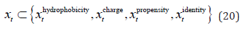
We investigated four features in our experiments. These features are commonly used, easy-to-extract and effective in producing high accuracy models [1,9]. They are:

Hydrophobicity of amino acids: This index of each amino acid type is obtained from Kyte and Doolittle hydrophobicity scale [10]. Table 1 shows the hydrophobicity index of each type of amino acid. The extracted feature is the mean of hydrophobicity of 10 residues before and after the predicted residue and itself:

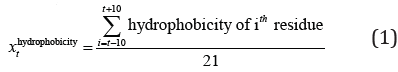
Table 1: Amino acid hydrophobicity scale.

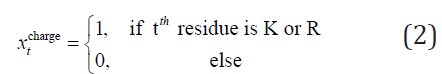
Positive charge of amino acids: The feature has value 1 with residue K-Lysine and R-Arginine and value 0 with the rest because K and R are the only two positive charge residues. This feature was used based on the “Positive Inside Rule”: connecting ‘loop’ regions on the inside of the membrane have more positive charges than ‘loop’ regions on the outside [11]. This information provided us clues about positions of transmembrane regions on proteins. This feature is expressed as:

Propensity of amino acids: This index is a statistical result obtained from the entire SWISS-PROT database and it was used as a feature in PRED-TMR method [12,13]. Table 2 shows the propensity index for each type of amino acid. The index was calculated by the formula:

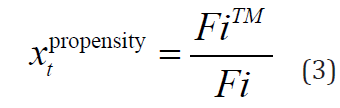
Table 2: Amino acid propensity value (transmembrane potential).

Where i is the type of t^th residue; Fi^TM and Fi are the frequencies of the type i residue in transmembrane segments and in the entire SWISS-PROT database respectively.

Identity of amino acids: This feature is a vector of 20 in length. Each amino acid is expressed by value 1 at its corresponding element and 0 at the rests:

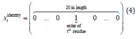
The assigned order of amino acid type is shown in Table 3.

Table 3: Assigned order of amino acids.

Methodology

Figure 1: System flow chart.

In this paper, we proposed a new approach using Long Short- Term Memory (LSTM) [14] model. LSTM is a recurrent neural network structure that has the ability to learn relationships between far sequential samples. Although neural network model has been used before [2], the range of surrounding residues (in a sliding window) that was analyzed to predict the center residue was very limited. Particularly, only 10 residues before and after the predicted residue were included in the window. To increase the analyzed range of surrounding residues, we have to increase the size of the sliding window which increases the number of nodes in the whole neural network. This disadvantage stops our model from learning relationships between far amino acids. However, with the recurrent structure of LSTM, we can capture the relationship between unlimitedly far residues without increasing the structure’s size. With this advantage, we expect our model to give more correct predictions about the transmembrane structure of protein. We can use information from nearby residues in both sides of the predicted residue to give better predictions. Therefore, a bidirectional LSTM model was used to learn the relationship of one residue with its nearby residues from both sides. Figure 1 demonstrates the flow chart of our system.

Model configuration

Figure 2: Our bidirectional LSTM.

Since we wanted to investigate the effect of each feature on the system’s performance, we implemented our model using different combinations of features along with different configurations. For each direction of the bidirectional LSTM, our structure had one layer with the number of hidden units varying according to the used combination of features. For each feature combination, we had tried many values of number of units to find the best configuration. For all combinations consisting of propensity feature (whose length of feature vector is 20), 150 hidden LSTM units were used, and other cases not consisting of this feature, 50 units were used. Each LSTM unit had a recurrent connection to itself and all the units in the same layer. We used the full standard configuration of LSTM which had input, output, forget gates and peephole system. For each amino acid, results returned from the two-directional LSTMs were summed up and then propagated to an one-layered feed forward network. This feed forward network had two units in the output layer, indicating the probability of the residue to be transmembrane or not. The learning rate used for all cases was 0.01, and the cost function was a cross-entropy function. Figure 2 demonstrates the used bidirectional LSTM. Formulas (5) to (19) describes this model mathematically.

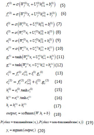
• xt : input feature of the tth amino acid.

• f_t(1) , i_t(1) , o_t, g_t(1) , c_t(1) , h_t(1) ,: the values of forget gate, input gate, output gate, candidate value, cell state and hidden state respectively of the first LSTM (forward LSTM) at the tth amino acid.

• W_f⁽¹⁾ , U_f⁽¹⁾ , b_f⁽¹⁾ , W_i(1) , U_i⁽¹⁾ , b_i⁽¹⁾ , W₀⁽¹⁾ , U₀⁽¹⁾ , b₀⁽¹⁾ , W_g⁽¹⁾ , U_g⁽¹⁾ , b_g⁽¹⁾ : weights and bias of the above mentiond values.

• f_t⁽²⁾ , i_t⁽²⁾ , o_t⁽²⁾ , g_t⁽²⁾ , c_t⁽²⁾ , h_t⁽²⁾: values of forget gate, input gate, output gate, candidate value, cell state and hidden state respectively of the second LSTM (backward LSTM) at the tth amino acid.

• W_f⁽²⁾ , U_f⁽²⁾ , b_f⁽²⁾ , W_i⁽²⁾ , U_i⁽²⁾ , b_i⁽²⁾ , W_o⁽²⁾ , U_o⁽²⁾ , b_o⁽²⁾ , W_g⁽²⁾ , U_g⁽²⁾ , b_g⁽²⁾ : weights and bias of the above mentiond values.

• σ , tanh, softmax: logistic, hyperbolic tangent and softmax activation function, respectively.

• h_t : sum of outputs from two LSTMs at the t^th amino acid.

• W, b output_t : weights and bias of the dense layer and its output at the t^thamino acid.

• y_t : prediction from our model, the probability indicating whether the t^th amino acid is transmembrane or not.

Post-processing

Although prediction accuracy returned from the bidirectional LSTM might have been high, we still aimed to improve by a postprocessing step. Actually, this step might reduce slightly the prediction accuracy on amino acids (only less than 0.3%). However, it improved accuracy in detection of transmembrane regions overall, which was our main objective. The rules for post-processing were:

a. Dividing too long transmembrane-predicted region (more than 30 residues) into two regions with same lengths by changing the middle residue into non-transmembrane residue

b. Rejecting too short transmembrane region (less than 5 residues) by changing all of its residues into nontransmembrane residues

c. Connecting two predicted transmembrane regions if they were divided by one non-transmembrane residue and sum of the length of two regions was less than 25. We did this by changing the dividing non-transmembrane residue into a transmembrane residue.

Results and Discussion

Go to

• Abstract
• Introduction
• Materials and Methodology
• Results and Discussion
• Results
• Discussion
• Conclusion
• References

Experiments

In order to investigate the effect of the mentioned features on the performance of our predictions, we implemented the LSTM model with different combinations of them. To be more specific, we implemented the model with each feature separately and all combinations of two, three and four features. Therefore, the mathematical formula of a sample’s feature was:

Because these features have different lengths (1 for hydrophobicity, positive charge, propensity feature and 20 for identity feature), so for each combination, we had tried and chosen the best LSTM configuration (number of hidden units) as mentioned in the model configuration section. Note that the predictions returned by the bidirectional LSTM were not postprocessed since we aimed to assess the raw performance of each feature combination.

To compare the quality of our model with other methods, we also tested common available transmembrane region predictors: Rost et al. [2], Krogh et al. [3], Hirokawa et al. [15] on our testing dataset. Systems of these methods are implemented on web servers at [16] for PHDhtm, [17] for Hirokawa [15,18] for SOSUI. According to review articles [1,19], these are considered good predictors which used a variety of approaches. Indeed, comparison result in [19] indicated that TMHMM, which employed hidden Markov model to predict transmembrane region, is so far the best transmembrane helix predictor. PHDhtm and SOSUI are two methods using different approaches from us which were vanilla neural network and hydrophobicity analysis - a non-machine-learning method, respectively.

In this comparison, our model used the combination of three features, namely hydrophobicity, propensity, and positive charge:

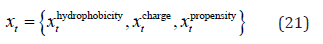
In this comparison test, we also used the post-processing step to improve accuracy of our model. All the experiments were implemented on a Dell PC with configuration: an Intel(R) Core(TM) i7-6700K CPU, 24GB of RAM and an NVIDIA GeForce GTX 750 Ti GPU.

Results

Go to

• Abstract
• Introduction
• Materials and Methodology
• Results and Discussion
• Results
• Discussion
• Conclusion
• References

The tesing results of LSTM models using different combinations of features are shown in Table 4-7.

a. Each feature: (Table 4)

Table 4: Assigned order of amino acids

TP_amino acid: Percentage of correctly predicted transmembrane residues (true positives).

TN_amino acid: Percentage of correctly predicted non-transmembrane residues (true negatives).

CP_amino acid: Percentage of correctly predicted transmembrane and nontransmembrane residues (correct predictions).

b. The test results of our model and comparing models (PHDhtm, TMHMM and SOSUI) are shown in Table 8.

Discussion

Go to

• Abstract
• Introduction
• Materials and Methodology
• Results and Discussion
• Results
• Discussion
• Conclusion
• References

According to Table 4, the features hydrophobicity, propensity, and identity had already worked well on their own. In particular, they gained higher than 90% of correct predictions on residues. Notice that although the identity feature did not rely on any physical or chemical characteristic of a residue, it still produced high accuracy predictions. By contrast, the positive charge feature did not work well. Indeed, it just produced about 75% of correct predictions.

Combinations of these features increased the accuracy remarkably as shown in Table 5-7. Figure 3 illustrates the average accuracies of combinations of one, two, three, and four features. Combinations of more features tended to produce higher accuracies. However, not all combinations of more features would produce higher accuracies, as in the case of the combination of propensity and positive charge comparing to the combination of hydrophobicity, propensity, and identity. A reasonable explanation for this exception is the used LSTM configurations might not have been the best configuration for the corresponding combinations of features. When comparing with other state-of-the-art methods, we chose the set of features: hydrophobicity, propensity, and positive charge. Since this set of features produced high accuracy - approximately 92.56%, and used only three features.

Table 5: Experimental results of combinations of two features.

Table 6: Experimental results of combinations of three features.

Table 7: Experimental results of combinations of four features.

Figure 3: Accuracies comparisonbetween combinations of features.

We also observed that the combination of identity, propensity, and positive charge has the highest true positive prediction accuracy-TPamino acid (82.76%). Thus if we do not want to miss any transmembrane residue, this combination would be a reasonable choice to use. On the other hand, the combination of hydrophobicity, and positive charge has the highest true negative prediction accuracy-TNamino acid (96.57%), and therefore should be used when we want to avoid predicting any non-existing transmembrane region.

Results in Table 8 indicated that our method’s accuracy is as high as other predictors, and even higher than some of them. Indeed, the bidirectional LSTM method is better than all others in some aspects: true negatives (TNamino acid) and correct predictions (CPamino acid) of predicted residues, true positives (TPregion) and false positives (FPregion) of predicted regions.

Table 8: Experimental results of combinations of four features.

TP_region: Percentage of correctly predicted transmembrane regions (true positives). A predicted transmembrane region is considered correct if it overlaps at least 10 residues with the ground truth transmembrane region.

Conclusion

Go to

• Abstract
• Introduction
• Materials and Methodology
• Results and Discussion
• Results
• Discussion
• Conclusion
• References

In this study, we introduced a novel approach to predicting transmembrane region on proteins using a bidirectional LSTM model. Experiments showed that our system was better than other state-of-the-art methods in following aspects: true negatives and correct predictions of predicted residues, true positives and false positives of predicted regions. Furthermore, we investigated the effect of each used feature. Results indicated that models using one of the features: identity, propensity and hydrophobicity had already produced high accuracies. When combining these features with residue charge feature or with each other, the accuracies rose noticeably.

References

Go to

• Abstract
• Introduction
• Materials and Methodology
• Results and Discussion
• Results
• Discussion
• Conclusion
• References

1. Chen CP, Rost B (2002) State-of-the-art in membrane protein. Appl Bioinformatics 1(1): 21-35.
2. Rost B, Fariselli P, Casadio R (1996) Topology prediction for helical transmembrane proteins at 86% accuracy. Protein Sci 5(8): 1704-1718.
3. Krogh A, Larsson B, Heijne GV, Sonnhammer ELL (2001) Predicting transmembrane protein topology with a hidden markov model: Application to complete genomes. J Mol Biol 305(3): 567-580.
4. Tusnády GE, Simon I (2001) The HMMTOP transmembrane topology prediction server. Bioinformatics 17(9): 849-850.
5. Yuan Z, Mattick JS, Teasdale RD (2004) SVMtm: support vector machines to predict transmembrane segments. J Comput Chem 25(5): 632-636.
6. Möller S, Kriventseva EV, Apweiler R (2000) A collection of well characterised integral membrane proteins. Bioinformatics 16(12): 1159-1160.
7. Möller S, Kriventseva EV, Apweiler R (2016) Collection of well characterized integral membrane proteins.
8. Krogh A, Larsson B, Heijne GV, Sonnhammer ELL (2016) Training dataset of TMHMM.
9. Punta M, Forrest LR, Bigelow H, Kernytsky A, Liu J, et al. (2007) Membrane protein prediction methods. Methods 41(4): 460-474.
10. Kyte J, Doolittle RF (1982) A simple method for displaying the hydropathic character of a protein. J Mol Biol 157(1): 105-132.
11. vonHeijne G, Gavel Y (1988) Topogenic signals in integral membrane proteins. European Journal of Biochemistry. 174(4): 671-678.
12. Pasquier C, Promponas VJ, Palaios GA, Hamodrakas JS, Hamodrakas SJ (1999) A novel method for predicting transmembrane segments in proteins based on a statistical analysis of the SwissProt database: the PRED-TMR algorithm. Protein Eng 12(5): 381-385.
13. (2016) Propensity of amino acid.
14. Hochreiter S, Schmidhuber J (1997) Long short-term memory. Neural Computation 9(8): 1735-1780.
15. Hirokawa T, Boon CS, Mitaku S (1998) SOSUI: classification and secondary structure. Bioinformatics 14(4): 378-379.
16. Rost B, Fariselli P, Casadio R (1996) PHDhtm server.
17. Krogh A, Larsson B, Heijne GV, Sonnhammer ELL (2001) TMHMM server.
18. Hirokawa T, Boon CS, Mitaku S (1998) SOSUI server.
19. Möller S, Croning MD, Apweiler R (2001) Evaluation of methods for the prediction of membrane spanning regions. Bioinformatics 17(7): 646- 653.
20. Chen CP, Rost B (2002) State-of-the-art in membrane protein. Applied Bioinformatics 1(1): 21-35.
21. Pasquier C, Hamodrakas SJ (1999) An hierarchical artificial neural network system for the classification of transmembrane proteins. Protein Engineering, Design & Selection 12(8): 631-634.

© 2018 PhamThe Bao. This is an open access article distributed under the terms of the Creative Commons Attribution License , which permits unrestricted use, distribution, and build upon your work non-commercially.