The “Reversal” of the Relative Age Effect

This paper develops a stochastic selection model that describes the processes related to the relative age effect in sports. The model helps to explain why the relative age effect exists. In addition, some distribution theory related to the model allows the quantification and comparison of the expected performance of athletes having early and late birth dates in elite sports. The latter derivation helps to explain the so-called “reversal” of the relative age effect.

Keywords: Relative age effect; Selection bias; Statistical modelling

The relative age effect in sport is the phenomenon whereby a disproportionate number of athletes at the highest levels of team competition have birthdays that fall early in the year. A basic explanation for the relative age effect is that athletes are first selected for elite training while they are young. A common selection process involves a comparison of children from a given birth year. Naturally, those born in the early months (say, January and February) are older. On average, they are also more physically advanced and advantaged than those born in the later months (say, November and December). Therefore, selection for participation on elite teams will tend to favor children born early in the year. Consequently, advanced training provides a continual advantage that is difficult for unselected athletes to overcome, and a cycle is imposed during career development that favors athletes born early in the year. The relative age effect in sport appears to have been first identified in ice hockey [1], and since that time, research on the relative age effect has flourished across various disciplines. The topic has even gained interest in the public sphere where it has been discussed in the popular book “Outliers” [2]. Two primary threads of investigation involving the relative age effect are: (i) its existence in particular sports (e.g., in American football [3], soccer [4], and baseball [5]), and (ii) remedies to counter the relative age effect [6,7].

Another line of research related to the relative age effect concerns the reversal of the relative age effect (see, for example, Fumarco et al. [8], Ramos-Filho and Ferreira [9], Gibbs et al. [10], and McCarthy et al. [11]). For this author, the term “reversal” is viewed as possibly misleading terminology, as the term may suggest that the relative age effect no longer exists. In fact, the relative age effect continues to exist in many sports. What the literature intends to convey by the term “reversal” is that once athletes reach the highest levels of team sport, meaningful differences no longer exist in the abilities and performance between those who are born early in the year and those born late in the year. Some papers (e.g., Fumarco et al. [8]) even suggest that those born later in the year may surpass those who were born earlier in the year. For some, this could be viewed as a paradox.

A growing and widespread emphasis in sports now involves equity, diversity and inclusivity (EDI) [12]. The relative age effect is an example of a lack of equity, as younger athletes (in the selection year) are disadvantaged in terms of achieving elite status in their sport. Again, the messaging that the relative age effect has been reversed may cause some to think that the problem no longer exists. Nevertheless, the relative age effect remains a problem from an equity viewpoint. Some evidence also indicates that those born in later months may be disadvantaged in other ways, including in their education [13].

In Section 2, a selection model is proposed that describes the basic features related to participation in elite-level sports. It accommodates the steps involved in reaching various stages in a sport and introduces a parameter that describes athlete maturity. In Section 3, the selection model is analyzed, and the relative age effect is immediately apparent. A more detailed distribution theory provides an analytic expression for the expected performance of those athletes who advance to the next step in an elite sport. The expected performance formula is instructive for comparing those athletes who are born early versus those who are born late in the selection year. It is then apparent that the so-called “reversal” of the relative age effect is a natural consequence of full maturation. We then conclude with a short discussion in Section 4.

The Selection Model

In sport selection, the selection is often based on the calendar year. However, in some sports (e.g., UK football), the selection year begins on September 1 with the oldest cohort and ends the following August 31 with the youngest cohort. We present selection generically, and for simplicity, we denote H1 as the oldest cohort (i.e., the first half of the year) and H2 as the youngest cohort (i.e., the second half of the year). Other discussions involving the relative age effect often differentiate the year according to four birth quartiles.

Let t = t0, t1, . . . , tn denote the selection times during an athlete’s career, where the final selection time tn corresponds to the athlete’s entrance into the top league. For illustration, in hockey, this would involve the time of the entry draft in the National Hockey League (NHL). Not every player under consideration in the NHL draft is the same age; however, we make this simplifying assumption. Importantly, t0 represents the time corresponding to selection at the earliest stage. For ice hockey in Canada, this often corresponds to “rep” teams involving 8-year-olds [14].

Based on a nearly uniform birth distribution throughout the year [15], we assume an initial pool of =N potential athletes in H1 and an initial pool of potential athletes in H2. In general, we let be the number of H1 athletes and we let be the number of H2 athletes available for selection at time t. Further, let denote the performance of athlete j from H1 at time t, j = 1,…, and let denote the performance of athlete j from H2 at time t, j = 1,…, .Without loss of generality, we let large values of X denote strong performance. The performance ranking is some sort of aggregate ranking for a player upon which selection at the next level is determined. For the purposes of our theoretical development, the quantity does not need to be fully defined. However, for example, at the NHL draft, the performance ranking could simply be the inverse draft order; that is, we assign performance rank 224 to the first player drafted we assign performance rank 1 to the 224-th (last) player drafted, and we assign performance rank 0 to all undrafted players. Using the above notation, we define the stochastic model as

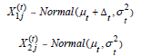
In (1), the parameter represents the mean level of players at time t where improvement over time is expressed via the constraint 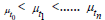The parameter represents the advantage that the older cohort H1 receives due to a maturation advantage. This could be a function of various factors including anthropometric, physical, physiological, emotional and cognitive advantages. Maturation advantages naturally dissipate over time, and this is expressed via .

The final component in the selection model is the threshold for advancement. We define a threshold ct at time t whereby athlete j advances to the next level if for cohorts i = 1, 2.

The model (1) and the advancement mechanism are simple constructs that capture the main features of the selection process in a sport. Of course, there are many nuances that could be built into the model such as a participant’s choice to leave the sport that is not related to performance. As another example, a factor that favors late-born athletes could be introduced, as suggested by McCarthy et al. [11]. We see that participation in sports may be viewed as a triangle with a broad base of participants. As time progresses, fewer players move up the triangle (i.e., advance) until very few are left at the top echelon of a sport.

Given model (1) and the advancement mechanism described in Section 2, we now investigate two consequences related to the relative age effect.

Existence of the relative age effect

Without loss of generality, consider the very first step of advancement at time t0. According to the model developed in Section 2, advancement occurs for athlete j in cohort H1 if

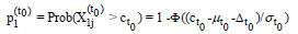
Where Φ is the cumulative distribution function of the standard normal distribution. Similarly, advancement occurs for athlete j in cohort H2 if and this occurs with probability

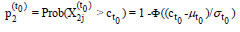
Since the expressions (2) and (3) imply that . Further, since the number of athletes who advance to the next level are and 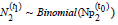, respectively, it follows that

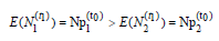
In other words, from (4), the expected number of athletes who advance from H1 exceeds the expected number of athletes who advance from H2; this is precisely the relative age effect.

“Reversal” of the relative age effect

Consider now athlete j who has made it to the most elite stage. For cohort H1, this Means and for cohort H2, this means . With the athlete having reached the most elite stage, we are now interested in a comparison of the expected performance between the two cohorts. Using distribution theory related to the standard normal distribution, we can show that the relevant conditional expectations are given by:

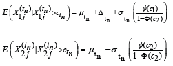
Where 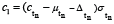and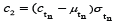

Therefore (5) provides an analytic expression which permits investigation of the conditional expectations where the terms in parentheses are the well-studied inverse Mills ratios [16].

In particular, it can be shown that 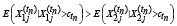which casts doubt on the claim of reversal of the relative age effect. However, we recall that maturation advantages dissipate over time Therefore, if we assume then the two conditional expectations are identical, and we establish reversal of the relative age effect.

This short communication develops a stochastic selection model that describes the process of player selection at different stages of development. The model is relatively simple and contains assumptions that appear to be common across various team sports. The model can explain the relative age effect. In addition, the distribution theory associated with the model can explain the so-called “reversal” of the relative age effect, where, at advanced stages, the expected performance differences no longer occur between younger and older athletes from the same age cohort.

Future research may consider enhancement of the model to reflect nuances inherent in particular sports. With increased availability of data, the parameters of the model may be estimated, and greater insights may be attained. Having a theoretical structure is beneficial, as it permits broader study of the relative age effect.

T. Swartz is Professor, Department of Statistics and Actuarial Science, Simon Fraser University, 8888 University Drive, Burnaby BC, Canada V5A1S6. Swartz has been partially supported by the Natural Sciences and Engineering Research Council of Canada. The work has also been partially support by a CANSSI (Canadian Statistical Sciences Institute) Collaborative Research Grant (CRT) in Sports Analytics.

1. Barnsley RH, Thompson AH, Barnsley PE (1985) Hockey success and birthdate: The relative age effect. Can Assoc Phys Educ Recreat J 51: 23-28.
2. Gladwell M (2008) Outliers: The story of success. Little, Brown and Company, New York, USA.
3. Heneghan JF, Herron MC (2019) Relative age effects in American professional football. J Quant Anal Sports 15(3): 185-202.
4. Yague, JM, de la Rubia A, Sanchez-Molina J, Marota-Izquierdo S, Molinero O (2018) The relative age effect in the 10 best leagues of male professional football of the Union or European Football Associations (UEFA). J Sports Sci Med 17(3): 409-416.
5. Thompson AH, Barnsley RH, Stebelsky G (1991) “Born to play ball”: The relative age effect and Major League Baseball. Sociol Sport J 8(2): 146-151.
6. Hurley W, Lior D, Tracze S (2001) A proposal to reduce the age discrimination in Canadian minor hockey. Can Public Policy 27(1): 65-75.
7. Webdale K, Baker J, Schorer J, Wattie N (2020) Solving sport’s “relative age” problem: A systematic review of proposed solutions. Int Rev Sport Exerc Psychol 13(1): 187-204.
8. Fumarco L, Gibbs BG, Jarvis JA, Rossi G (2017) The relative age effect reversal among the National Hockey League elite. PLoS ONE 12: e0182827.
9. Ramos-Filho L, Ferreira MP (2021) The reverse relative age effect in professional soccer: an analysis of the Brazilian National League of 2015. Eur Sport Manag Q 21(1): 78-93.
10. Gibbs BG, Jarvis JA, Dufur MJ (2012) The rise of the underdog? The relative age effect reversal among Canadian-born NHL hockey players: A reply to Nolan and Howell. Int Rev Sociol Sport 47(5): 644-649.
11. McCarthy N, Collins D, Court D (2016) Start hard, finish better: further evidence for the reversal of the RAE advantage. J Sports Sci 34(15): 1461-1465.
12. Dashper K (2013) Introduction: diversity, equity and inclusion in sport and leisure. Sport Soc 16(10): 1227-1232.
13. Solli IF (2017) Left behind by birth month. Educ Econ 4(4): 323-346.
14. Hockey Canada Age Divisions (2020).
15. Melina R (2010) In which month are the most babies born? LiveScience.
16. Grimmett G, Stirzaker S (2001) Probability theory and random processes. (3^rd edn), Cambridge Publishers, Cambridge, USA.