LIDAR Monitoring of Urban Areas

The use of a LIDAR to monitor the air pollution makes it possible to control large city areas and detect the spatiotemporal location of Particulate Matter (PM) emissions sources. LIDAR monitoring is a fast method for estimating the pollution, respectively the mass concentration of PM in the atmospheric ground bioaerosol. The careful study of air pollution becomes especially relevant as the PM are potential carriers of solid-state particles dangerous to health and biologically active components. The present report summarizes our experience [1-3] on how the intricate complex of particles with different content and size found in the aerosol might affect the LIDAR monitoring results on the long distance. LIDAR subject of this study is capable of scanning and mapping the horizontal and vertical aerosol distributions and the transport of air masses with a range resolution along the Line of Sight (LOS) of 30m and a beam divergence of ~1 mrad at operational distances of about 25km [3]. The laser emitter (wavelength of 510.6nm) is a pulsed CuBr vapor laser with a repetition rate of 5-10kHz at a 15-ns pulse duration. The receiving system comprises a Carl Zeiss Jena Cassegrain telescope (aperture of 20cm and a focal distance of 1m), a 2-mm-wide focal diaphragm, an interference filter with a 2-nm-wide passband, and an EMI 9789 photo-multiplier tube operating in a photon-counting mode along the entire operational distance. The receiving system is fully computerized for collecting and processing the LIDAR data using a PCO 1001 1024-channel digital interface system for signal strobing and accumulation. The LIDAR monitoring was calibrated based on the data from a sampling absorber located just below the spot of the LIDAR beam with a flow rate of 100m3/h, where the particles are collected on a filter with pore size 3μm (FILTER-LAB, Material MCE, Lot.180509006).

Lidar monitoring

Analyzing the PM in aerosol loadings formed in the vicinity of the near surface level of the atmospheric urban areas and the experimentally aerosol data provided by the LIDAR technique two major LIDAR parameters have to be calibrated in terms of the aerosol mass concentration: (i) the extinction coefficient α(r) and (ii) the backscatter coefficient β(r). They can be determined by the well-known method [4,5] and making use of the mass concentration Ma data obtained by the sampling device. For the LIDAR ratio LiR = α(r)/β(r) we adopted the typical value of LiR=50 [6]. The parameters β(r) and α(r) were calculated using the LIDAR equation under the assumption of a horizontally-homogeneous atmosphere (1):

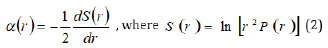
Where P (r) is the power of the detected laser radiation backscattered from the atmosphere from a distance r = ct/2 after a period of time t following the moment of laser pulse emission and is the pulse duration. Under the homogeneity assumption, the extinction coefficient α(r) is calculated as (2):

The calibration dependencies were developed of the mass concentration in [mg/m3] of α(r) and β(r). In both cases, the linear fit (Y = A + Bx) shows acceptable values of the standard deviation (less than 4%) and the correlation coefficient (over 0.92). The plots can be used directly for calibrating the LIDAR maps in mass concentration.

The LIDAR observation schedule complied with the generally accepted manner of measuring the aerosols mass concentration by air-quality monitoring systems. The sampling device pumps the atmospheric air through the filter (typically a volume of 600m3) for an interval of about a few hours. Thus, the laser beam was stationary and directed to pass above the aspirator at a height of hPM<δR, δR ̴30, being the LIDAR’s radial resolution. The height of placing the aspirator was also chosen to comply with this condition hasp < δR. LIDAR signals represent the number of backscattered photons Lphot (k.δR,τm), where k=1.Kmax, Kmax = Rmax/ δR, and τm=5min is the time of photons accumulation. The total time of measurement lasted from one to several hours, depending on the particular weather situation. The computer system processes the input data by solving the LIDAR equation (1), with its output being profiles of the backscatter coefficient β (k. δR ) or the extinction coefficient ε(k. δR ), as calibrated in terms of aerosols mass concentration. The set of LIDAR profiles obtained for the entire period of measurement is used to construct 3D LIDAR maps, with the x axis presenting the accumulation time with a step of τm=5min and the y axis, the distance from the LIDAR with a step at δR. The axis z corresponds to the coefficients of the backscatter or the extinction. The stability of the LIDAR parameters and consequently, the long-term calibration stability of the measurements results are of great importance in expecting reliable comparison of the LIDAR-measured atmospheric parameters, namely, the extinction & backscattering coefficients, or the attenuation of the LIDAR radiation along the remotely probed directions covering practically the entire city area of basic interest [4].

The correlation coefficient of the fitted plot is varying also within the too high and too close limits of 0.99 to 0.96. Figure 1 illustrates the PM mass concentration measurement in the LIDAR experiment on 19.05.2020 based on the backscattering coefficients. The measurements were conducted in the dark part of the day from 20:00 to 22:00. The inset shows the data at a time of greatest traffic for PM measured during the experiment. The LIDAR data were similar to the measured data of a mobile devices sampling in the path of the LIDAR beam. In situ sampling was performed simultaneously with the remote sensing using the sensor SDS 011 mobile device, filter absorber mentioned above, and data was compared with those of the municipality stationary station data for PM10. The data of the SDS 011 are lower (about 3.8%) and this is due to the difference in the volumes of the tested aerosol.

Figure 1: Lidar monitoring along a horizontal of the laser beam path based on the backscattering coefficients on 19.05.2020 from the 0 point - the lidar station.

The application of the LIDAR-based remote sensing technologies could be successfully used for direct and fast control of the averaged PM pollution including their mapping over large city areas. It was demonstrated by specific sets of target experiments that the LIDAR monitoring provides promising opportunities for an identification of PM mass concentration if processing of some of the basic LIDAR parameters as the extinction & backscattering coefficients, characterizing the interaction of the laser radiation with PM. The use of a single-frequency laser makes the method easy to implement, but does not allow to distinguish the dimensions of the PM. These necessities the combination of LIDAR monitoring with mobile devices or stationary stations for in situ sampling so that monitoring can provide in addition to quantitative data and qualitative information for the spatio-temporal distribution of pollution.

This work was financed under contract DN18/16 with the National Science Fund, Bulgaria, and included in the European Program of the COST CA16202.

1. Stoyanov D, Nedkov I, Grudeva V, Cherkezova-Zheleva Z, Grigorov I, et al. (2019) Long distance LIDAR mapping schematic for fast monitoring of bioaerosol pollution over large city areas. Atmospheric Air Pollution and Monitoring. Lakhouit A (Edr.), ISBN: 978-1-78985-280-6, Publ. Intech Open, London.
2. Angelova B, Iliev M, Ilieva R, Grigorov I, Kolarov G, et al. (2020) Complex study of the bioaerosol composition of the atmpsphere over urban areas based on lidar monitoring during the quarantine COVID-19. Machines Technologies Materials (7): 272-276.
3. Peshev ZY, Dreischuh TN, Toncheva EN, Stoyanov DV (2012) Two-wavelength lidar characterization of atmospheric aerosol fields at low altitudes over heterogeneous terrain. J Appl Remote Sens 6(1).
4. Fernald F (1984) Analysis of atmospheric LIDAR observations: some comments. Appl Opt 23(5): 652-653.
5. He T, Stanič Y, Gao S, Bergant F, Veberič K, et al. (2012) Tracking of urban aerosols using combined LIDAR-based remote sensing and ground-based measurements. Atmos Meas Tech 5: 891-900.
6. Klett J (1981) Stable analytical inversion solution for processing LIDAR re Appl Opt 20(2): 211-220.