About Application of the Overset Grid Method for Fluid Structure Interaction Problems in 3D Codes Based on Modification of Godunov Scheme Uniform for Both CFD and CSD

To model both the dynamics of fluids and solids high-order accuracy modification of Godunov scheme in Euler-Lagrange variables is used. The improving of the accuracy of the scheme is achieved on compact 3*3*3 stencil by using space and time-dependent Riemann's solver. The same solver is used to calculate the interaction between fluids and solids (FSI problem). In the calculation process three types of difference overset grids are used. The first is a mobile surface grid in the form of a continuous set of triangles (STL file), which defines and accompanies the computational bodies, and two kinds of 3D rectangular grids. The second is the basic Cartesian fixed grid embedded in each body, and the third type of grid is the movable local Euler-Lagrangian grid associated with each triangle of the first surface grid, which also accompany the contact boundaries. The physical quantities in these grids are connected by mutual interpolation. A detailed description of the procedure was given in [1,2].

This 3D codes does not require complex 3D mesh generators, to start calculations for the user it is enough only to define the surfaces of the calculating objects as the STL files, which can be created by tools of engineering graphics. Application of these overset grids is convenient to simulate strong shock wave loading processes of moving deformable solids. Three-dimensional processes of interaction of detonation waves with elastic plastic bodies located near the charges are considered. The bodies (cylinders, cubes, tetrahedrons) are strongly and irreversibly deformed, the streams of detonation products move much faster, and gas jets are formed around the deforming bodies. The processes of propagation of detonation waves from the initiation zones of explosives and the effect of nonlinear behaviour of the material and the deforming of bodies on contact forces and the interaction process are taken into account. The strong influence of geometry, initial position and density of the deformable bodies is demonstrated.

Defining system of equations

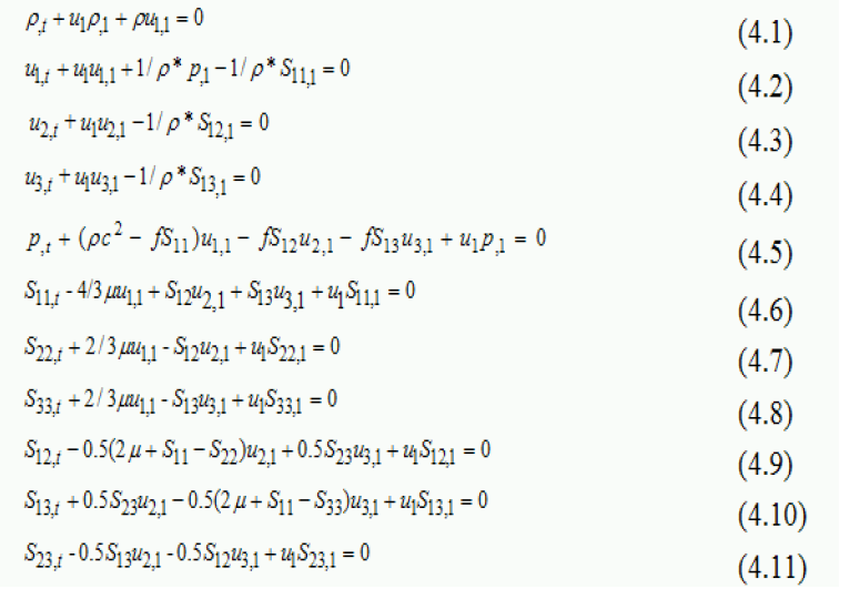
The closed system of equations describing the deformation of a continuous medium in the approximation of a model of a compressible elastoplastic body in the Cartesian coordinate system has the following form [3]:

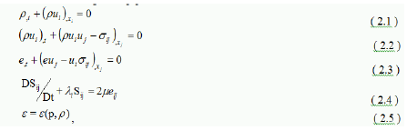
Notation: t-time, x_i-spatial coordinates, u_i-components of the velocity vector along the axes x_i respectively, p- density, 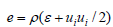- total energy per unit volume, - internal energy per unit mass, given by the equation of state (2.5), - which is represented as a ball and deviator parts, deviator of strain rate tensor 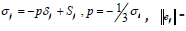- deviator of strain rate tensor . The symbol D/D denotes the Yaumann derivative, which takes into account the rotation of the stress tensor in Euler variables. 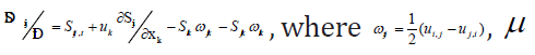, - is the material shear modulus, the index after the comma denotes differentiation with respect to the corresponding variable. As a criterion for the transition from the elastic to the plastic state, the von Mises yield condition under uniaxial tension is used, where - the yield stress under uniaxial tension. The parameter  must remain positive during plastic deformation under the condition of fluidity . The plastic flow is described by keeping the deviator on the surface of fluidity [3]. The system of Eq. (2.1) -(2.5) is closed by equations of state with the corresponding parameters. In the absence of shear stresses, system (2.1)-(2.5) obviously goes over to the Euler equations for the motion of a compressible gas. As a numerical method for solving equations (2.1)-(2.5), a modification of the Godunov scheme [4-6] is used, providing the second order of approximation on a compact 3*3*3 stencil. For the gas-dynamic part in comparison with the basic Godunov's scheme [7] changes are necessary to make only at the predictor step [6] when preparing parameters for the standard solution from [7].

Second order on compact stencil for CFD on moving Euler variable

The following technics is used to increase the accuracy of Godunov’s method:

Figure 1: Linear distribution of parameters (primitive for CFD, Riemann’s invariants for CSD) between cell’s centers.

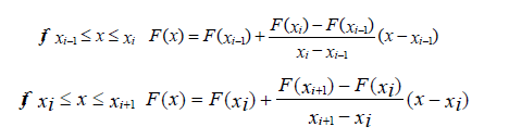
1. Assume all hydrodynamics parameters to be linearly distributed in space between the cell centers for all time steps, for example: for cell number i,j,k time step t_n in X direction, vector function F with scalar components  has such distribution (Figure 1).



2.  Riemann's problems (for example for cell number “ i “ with boundaries xi-1/2 and xi-1/2, are calculated for values F(x₁) F(x₂) and F(x₃) F(x₄), respectively. For original Godunov’s method these problems are solved for F(xi-1)F(x_i)and F(x_i)F(Xi+1)  values respectively. Points x1,x2 and x3,x4 are not known yet.
3. Flux calculation and the corrector step (integration) are exactly the same as in original Godunov's method.
4. Now the solution at the time step tn+1 is a function of hydrodynamics values of those points x1,x2  and x3,x4. For linearized Euler equations, it is possible to obtain Riemann’s solution and hydrodynamics parameters at the new time step as explicit functions of coordinates of these points.
5. Using an appropriate choice of these points it is possible to eliminate or to introduce the required viscosity terms into the differential equations. For the zero viscosity terms these points are physically meaningful.

Let us analyze for example the 1D linearized Euler equations:

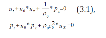
where p0,p0,u0 are points of linearization, c₀=c₀(p₀,p₀) ).

Using assumptions 1,2,3,4 and Taylor’s differential formulas in numerical integration of this cell number “i “, it follows from Eq. (3.1):

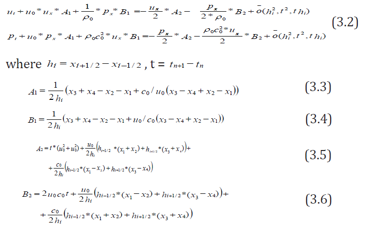
In Eq. (3.3-3.6) x₁, x₂, x₃,x₄  are taken relative to x_i; it means x_i=0. For simplification x₁,x₂  are taken relative to xi-1/2,and x3,x4- relative to xi+1/2 respectively.

For system of Eq. (3.2) to have the first order accuracy approximation error it is necessary that A₁=1; B₁=1  (3.7).

From Eq. (3.2) and (3.7) it follows that 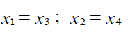(3.8)

For system of Eq. (3.2) to have the second order accuracy, it is necessary in addition to (3.7) to have A2=0; B₂=0  (3.9)

Then it follows from (3.7) and (3.9) that

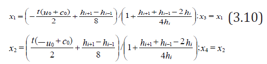
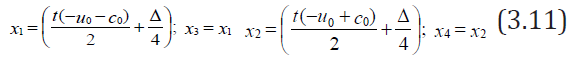
Formulas (3.10) show the coordinates of such points, the interpolation to which provides the second order accuracy approximation error of system of Eq. (3.2) for an irregular grid in this numerical method. For irregular grid it follows from (3.10) that the scheme obtained is not conservative. But for the usually used uniform or arithmetic progression grid, where 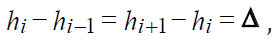, it is conservative, and formulas (3.10) assume the following form:

From Eq. (3.11) it is obvious that there is a shift to a bigger cell for the irregular mesh.

Figure 2: Linear distribution of parameters (primitive for CFD, Riemann’s invariants for CSD) between cell’s centers.

Eq. (3.10) and (3.11) for the interpolation point coordinates are very physical and have obvious geometrical interpretation (Figure 2). The zones of influence on the solution of Riemann's problem for the boundary of the cell at t/2 are restricted by these interpolation points. There is no difference between subsonic and supersonic cases. The algorithm is obviously extended to moving meshes-the zone of influence is calculated for moving boundary.

Second order on compact stencil for CSD on moving Euler variables

In modeling the elastic-plastic flows at the predictor step the elastic solution of the Riemann's problem is used, the plastic properties of the material are taken into account at the corrector step in accordance with [3], which provides the second order of approximation of the system of Eq. (2.1)-(2.5) as a whole.

Let us designate 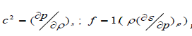, then, from the system of Eq. (2.1)-(2.5), by linearizing the energy equation to solve the Riemann's problem, eliminating terms containing derivatives with respect to  and we get the following system:

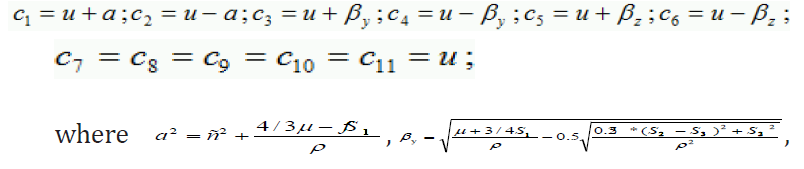
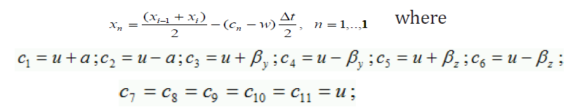
This system is hyperbolic and can be decomposed and using Riemann’s invariants written as 11 transport equations in the following form [4,5]:

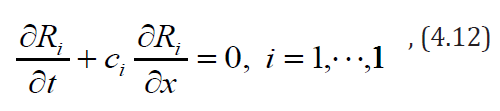
where is Riemann’s invariant, constant for appropriate characteristic velocity ,

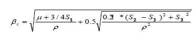
. For the Riemann’s solver for each zone of influence appropriate invariants coupled with appropriate cell’s center are taken (Figure 3). It provides first order accuracy.

To obtain the second order accuracy of approximation in the case of elastic-plastic flows it is assumed the linear distribution for Riemann’s invariants between cell’s centers (Figure 1). The Riemann’s invariants, which are used to obtain the primitive parameters of the Riemann’s solver, are to be determined by interpolation of appropriate invariants from the cell centers to the points from which the invariants of each family arrive the contact of neighboring cells (Figure 4). The appropriate points of interpolation are obtained in the following manner:

Figure 3: Characteristic plane of Riemann’s solver.

Figure 4: Zones of influence for Riemann’s solver for 2 order, where

Let us define the interpolated invariants with index ‘ ’, then 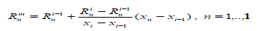. These values are used to define the primitive parameters of Riemann’s solver and appropriate fluxes of conservation laws and Hook’s law fluxes. The same solution is used to implement the basic boundary conditions: ‘rigid wall’-symmetric parameters are set with opposite normal velocity; “fixed boundary”- 3 velocity components on the boundary are specified, “pressure boundary”-normal stresses and zero shear stresses are specified. Free boundaries are a special case of “pressure boundaries”. Generally on the boundary instead of 3 invariants from the right side, 3 appropriate boundary conditions are taken.

Fluid structure interaction solver

The solution of the Riemann's problem for the three-dimensional case between an elastic medium and a gas (detonation products) is constructed similar [4,5] by an iterative combination of the nonlinear solution of the Riemann's problem for a rigid wall for gas [6,7] and “pressure boundary” for an elastic body. The gas interacts with the rigid wall having the velocity of the boundary of the elastic body, with the obtained boundary pressure “pressure boundary” for the elastic body is calculated. The obtained normal velocity of the boundary of the elastic body is used in the next iteration to calculate the interaction of gas with the rigid wall, and so on until convergence of the boundary velocity.

On monotonicity for modified scheme

 This high order scheme is not monotone. Despite the first order accuracy the main advantage of Godunov’s method is monotony for all kind of problems. The numerical viscosity of the original Godunov’s approach based on Riemann’s solution between cell’s centers is universal and enough for monotony. One of the aim of this modification is to keep this universal viscosity of the original Godunov’s method, reducing its viscosity. It is well-known that the problems with the monotony of the numerical solutions occur in the vicinity of the big gradients. More detailed analysis of the numerical results demonstrates that the origin of nonmonotonicity is not in the big gradients, but in the big rate of these gradients. So the nonmonotonicity problems are coupled with the regions where the behavior of the solution mainly depends from the second order derivatives. Physically these regions are at the top or at the bottom of acoustic or shock waves, density discontinuities and rarefaction waves. Mathematically they are around the points of the discontinuity of the first derivatives. Original Godunov’s method provides rather good behavior of the solutions in these regions and so to use the original Godunov’s predictor step as a universal method to cure our second order approach is rather simple and reliable way to avoid nonphysical oscillations. From the analysis of numerical results, obtained for this scheme, for monotony of the numerical solution in such rock generation regions, it is enough to use original Godunov’s predictor step for the one or two cell’s boundaries. The main problem is how to detect such boundaries. One of the way is to use two parabolic splines, constructed from the primitive variables (from pressure or normal stress) in the vicinity of the analyzed cell’s boundary, using three points, two points which are used for Riemann’s problem, and the nearest point to the left for the left spline and the nearest point to the right for the right spline. Such parabolic functions represent more precisely the behavior of numerical results. For example these spline functions can be not monotone in this interval when the numerical those are still monotone. In this case first order Riemann’s solver is to be taken. Also this criterion can be corrected in the way to decrease the choice of the first order Riemann’s solver. For CSD the spline function can be constructed only for normal component of stress tensor. The numerical experiments demonstrate the efficiency of this method to obtain monotonicity.

Conclusions on the modified scheme

This modification of Godunov scheme has second order accuracy in time and space for 3D ALE for both CFD and CSD (Euler and Euler-Cauchy equations) on compact 3*3*3 stencil. The improving of the accuracy of the scheme for both cases is achieved by using the 3D space and time-dependent Riemann's solver. Coupling of two Riemann’s solvers (nonlinear for gas and linearized for solids) is used to calculate the interaction between fluids and solids (FSI problem). For nonlinear behaviour of material for CSD splitting algorithm is used [3]. Splitting corrections are made after integration of linearized system of solids equations, keeping second order accuracy of approximation of the system.

Basic 3D FSI ALE model problem on the compact 3*3*3 stencil

Figure 5: Local ALE grid.

Figure 6: Before integration.

Using this modified scheme it is possible to calculate the following 3D FSI problem in ALE. Assume 3D rectangular mesh for solids (compact stencil 3*3*3, brown on Figure 5) and similar for fluid (green part on Figure 5). For these two compact stencils it is possible to integrate the cells of the core with second order accuracy. These cells are marked with crosses on Figure 6. On the boundary fluid-solids exact Riemann’s solver is used. This FSI boundary is moved with contact Lagrange velocity in normal to FSI surface to its final position for this integration time step (Figure 7). On other 5 boundaries Eulerian fluxes are calculated. For this model problem all volumes and surfaces are calculated exactly. It is ALE in 3D for FSI on these compact stencils with sharp interface. The integrated cells are marked with crosses (Figure 7).

Figure 7: After integration.

Multi mesh sharp interface method for 3D FSI

The method for calculating FSI in Euler variables can be attributed to multigrid algorithms of the Chimera type and Ghost Fluid Method (GFM) with Sharp Interface Method (SIM) [8-12]. In the calculation process three types of difference grids are used. The first is a mobile surface grid in the form of a continuous set of triangles (STL file). On Figure 8 there are two such grids, blue and red, defining two contacting bodies. With green and yellow colour the movable local Euler-Lagrangian grids of 3*3*3 cells associated with the surface grid are marked. Those are grids for 3D FSI ALE model problem. The number of these local grids is equal to the numbers of triangles of the surface grid. On the Figure 9 is the slice of the body with the basic Cartesian fixed grid embedded in the body. Four types of cubic cells for the computational domain are obtained: first- cells, cut by triangles of the domain’s surface, marked with green color (boundary cells), second- cell outside surface, third-cells inside the surface with the stencil which is enough for integrating them (marked with brown color), fourth-cells inside the surface without stencil to integrate them (marked with black point). Method of calculation of this 3D FSI problem consists of a sequence of the following steps:

Figure 8:

Figure 9:

1. The cells of the third type are integrated on the fixed Cartesian grid on the new time step.
2. From the Cartesian grid and local grids flow parameters are interpolated to local mobile grids, generated on the time step. For each local grid the model problem from par. VIII is solved (ALE step) and the flow parameters for the new time step are obtained for these core cells (boundary cloud).
3. Using the velocity at the center of each triangle derived from the Riemann’s solver of the model problem in step 2, the velocities at the vertices of each triangle of the surface are calculated and STL file of the surface is moved to the position on the new time. On Figure 10 the old position is marked with black color line, the new one-with red one.
4. The parameters on the new time step in the cells of the body on the new position for integrating of which there was no enough stencil (marked with black cross on Figure 10) are obtained using interpolation from the parameters of the main Cartesian grid and parameters of the boundary cloud (from step 2 integration results.
5. The new movable local Euler-Lagrangian grids associated with each triangle of the new surface grid are generated to start the next time step.

Figure 10:

Simulation of interaction of elastic-plastic bodies with the product of detonation

Figure 11: Computational domain.

On Figure 11 the statement of the problem is given. Charge of TNT-RDX TR 8530 of the spherical shape, radius 5cm, the source of initial detonation was set in a region of radius less than 0.2cm. The cross section passes through the center of the charge and the centers of the cubes. In the charge and the air the main grid was used with the side of the cubic cell 0.15cm. For the explosive, the parameters of the equation of state of the JWL type are taken from [13] as A=708.6056GPa, B=13.16457GPa, C=1.058238GPa, r₁=4.94, r₂=1.35, =0.28. The same state equation is used for air, air is assumed like product of detonation for Euler simulation without tracking the interface “detonation product”- “air”. Three steel cubes with side 1cm are marked with red color, the density is 7.8g/cm³, the bulk compression modulus is 1.75*10⁵GPa, the shear modulus is 8.077*10⁴GPa, the hardening modulus is 2.40*10²GPa, and the yield strength is 3.40*10²GPa, weight 7.8grams. Step of the main grid in cubes is 0.07cm. On Figure 12 the grids for steel and TNT is given. On Figure 13 & Figure 14 density distribution is presented at the beginning of process of FSI and at the moment of 55μs respectively. The cubes are strongly and irreversibly deformed, the streams of detonation products move much faster, and gas jets are formed around the cubes. On Figure 15 the shape of the cubes, respectively, at the initial moment and at 55μs are presented. On Figure 16 the shapes are presented for the initial moment and for 13 and 55μs. By 13μs the fragments practically acquired a residual form by slightly changing their position. On Figure 17 the residual form of the fragment flying along the axis of symmetry is shown in more detail, a depression has formed in the upper part, a bulge in the lower part, and the thickness along the symmetry axis has almost halved. Figure 18 shows the speed on time on the surface of the cube, accelerated in the vertical direction, the lower curve corresponds to the center of the upper surface (far from the charge), respectively, the upper curve-to the center of the lower surface of the cube (near to the charge). Similar simulations were made for cylinders and tetrahedrons. On Figure 19 and Figure 20 there are the residual forms of a cylinder and tetrahedron along the axis of symmetry. The following bodies of the equal mass of 0.92grams of the same steel, but of various shape, were also considered. These are tetrahedrons with a side of 1cm, disks with a diameter of 1cm, a height of 0.15cm and cubes with a side of 0.49cm, located at the same points. Figure 21 shows the dependence of the velocities of the center of mass on time for the disk (mark 1), tetrahedron (mark 2) and cube (mark 3), accelerated along the vertical axis. Dashed lines indicate these dependencies, calculated in an elastic formulation.

Figure 12: Mesh near the charge.

Figure 13: Density, beginning of FSI.

Figure 14: Density distribution at 55μs.

Figure 15: Density, beginning of FSI.

Figure 16: Density distribution at 13 and 55μs.

Figure 17: The residual form.

Figure 18: Velocity on the bottom and top of cube.

Figure 19: Residual form, cylinder.

Figure 20: Residual form, tetrahedron.

Figure 21: Velocities of various shape bodies in elastic and elastic plastic case.

The method allows simulate fluid structure interaction problems with big deformation and displacement in Euler variables. Calculations of the explosive effect of charges located near the deformable elements showed a significant effect of the FSI on the gas flow and deformation of the structure. The essential dependence of speed on the geometry of the bodies and changes in the shape of bodies during acceleration is obvious. The duration of the acceleration time of the bodies is comparable with the time of detonation wave exit to the contact surface. The basic residual deformations that change the geometry of the bodies occur at the initial stage of acceleration.

1. Abuziarov KM, Abuziarov MKh, Zefirov SVA (2014) Numerical technique for determining explosive loads in Euler variables on spatial structures during the detonation of solid explosives. Problems of Strength and Plasticity. Publishing house of the UNN, Russia, 76(4): 326-334.
2. Abuziarov KM, Abuziarov MKH, Kochetkov AV (2016) 3D fluid structure interaction problem solving method in euler variables based on the modified Godunov scheme. Materials Physics and Mechanics 28(1): 1-5.
3. Kukudzhanov VN (2004) The method of splitting of elastoplastic equations MTT. 1: 98-108.
4. Abouziarov M, Aiso H, Takahashi T (2004) An application of conservative scheme to structure problems. Series from Research Institute of Mathematics of Kyoto University. Mathematical Analysis in Fluid and Gas Dynamics 1353: 192-201.
5. Abouziarov M, Aiso H (2004) An application of retroactive characteristic method to conservative scheme for structure problems (elastic-plastic flows). Hyperbolic Problems, Theories, Numerics, Appli-cations. Tenth International Conference in Osaka, pp. 223-230.
6. Abuziarov MKh, Bazhenov VG, Kochetkov AV (1987) About a new effective approach to improving the accuracy of the Godunov scheme. Applied Problems of Strength and Ductility, pp. 43-49.
7. Godunov SK, Zabrodin AV, Ivanov MY, Kraiko AN, Prokopov GP, et al. (1976) Numerical solution of multidimensional problems of gas dynamics. Nauka, Moscow, Russaia.
8. Garimella R, Dyadechko V, Swartz В, Shashkov М (2005) Interface reconstruction in multi-fluid, multi-phase flow simulations. Proc 14^th Int Meshing Rоundtаble: 19-32.
9. Michael L, Nikiforakis N (2018) A multi-physics methodology for the simulation of reactive flow and elastoplastic structural response. Journal of Computational Physics 367(15): 1-27.
10. Glimm J, Li XL, Liu YJ, Хu ZL, Zhao N (2003) Conservative front tracking with improved accuracy. SIAM J Num Analysis 41(5): 1926-1947.
11. Abgrall R, Karni S (2001) Computations of соmрrеssiblе multifluids. J Comput Phys 169(2): 594-623.
12. Garimella RP, Fedkiw T, Aslam B, Merriman S, Osher (1999) A non-oscillatory Eulerian approach to interfaces in multimaterial flows (the ghost fluid method). J Com-put. Phys 152(2): 457-492.
13. (2002) Physics of the explosion/ed. L.P. Orlenko. T.1.2. Fizmatlit, Moscow, Russia.