Case Study: Frac-Hit Occurrence Prediction Using AI & ML

Due to the tightness of shale formations, production from these formations is dominantly a function of the contact between the horizontal well and the formation. Several clusters of hydraulic fractures and natural fracture networks are the main contributors to the contact between the well and the shale play. Since the natural fracture networks cannot be physically modeled due to their complexity and lack of measurement, physics-based modeling of Frac-Hits, a function of natural fracture networks, is also almost impossible. During the hydraulic fracturing of a child well, the extension of natural fracture networks that have been opened by the induced fractures can connect with the networks of natural fractures of the parent well. When the natural fracture networks of the hydraulic fracturing well known as child well communicate with the natural fracture networks existing well, parent well, Frac-Hit occurs. When Frac-Hit happens, the slick water injected in the child well will move through the connected networks of fractures and will be produced from the parent well.

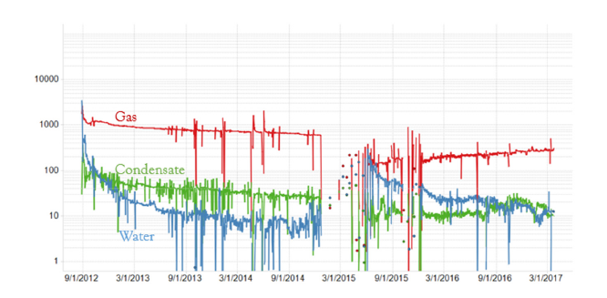
This increase in water production is usually accompanied by a reduction in hydrocarbon production in the parent well, negatively affecting the operator’s cash flow. Figure 1 shows the impact of Frac-Hit on the fluid production of a parent well where production of gas and condensate has dropped drastically in mid-2015 after Frac-Hit while water production has increased significantly located in southern Pennsylvania from Marcellus shales [6]. As the number of wells in a shale asset increases, reducing the spacing between wells and stacking wells in multiple layers as a common practice result in more interference between child and parent well known as Frac-Hit. Traditional approaches fail to predict, manage and mitigate Frac-Hit. The objective is modifying the traditional approaches by leveraging AI&ML techniques and replacing the assumptions currently used with a large amount of field measurements.

Figure 1:Impact of Frac-Hit on the production of the parent well, south PA [6].

In this article, two approaches of Frac-Hit prediction, mitigation and management are presented and one is discussed in detail:
a) Snapshot Modeling of Frac-Hit: Uses snapshots of the shale well dynamic behaviors to identify Frac-Hit, which is the focus of this article.
b) Dynamic Shale Analytics: Built on the top of Top-Down modeling technique and would be able to predict, manage and mitigate Frac-Hit through comprehensive dynamic profiles of all the shale assets [3].

The first AI/ML based approach, Snapshot Modeling of Frac- Hit, uses a snapshot in time of the dynamic behavior of the wells. This technique developed based on the work of a former graduate student at West Virginia University, Mr. Ryan Tyree, identifies two key parameters: First the contributing characteristics of reservoir, hydraulic fracturing and completion that cause the Frac-Hit. Second, predicting whether Frac-Hit will occur on the parent well during completion of the child well at stage level. The second AI/ML based approach, Dynamic Shale Analytics, uses a single model to history match the entire production profile of every single well in the asset, un-contrary of RTA or LSTM models that history match a single well. Moreover, the Dynamic Shale Analytics model incorporates several parameters in categories of construction and trajectory, hydraulic fracturing design, operational constraints and production history and unlike numerical reservoir simulation; the model simulates the combination of reservoir and the wellbore.

Figure 2:Casing pressure on the child well identifies the Frac-Hit from the child well [6].

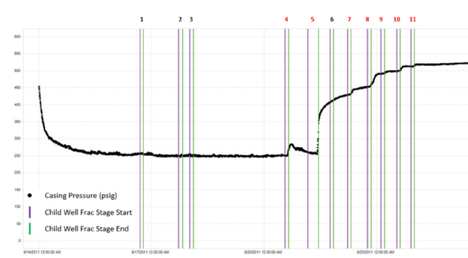
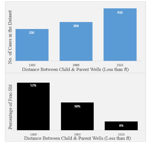
Data from 964 frac stages of 79 child wells in Marcellus shale assets covering an area of 112 squared miles located in southern Pennsylvania was used in this study. These child wells have the change to Frac-Hit on 63 parent wells in this dataset. The effect of each child’s well frac stage (Frac-Hit/No Frac-Hit) was then evaluated on the parent well. Figure 2 is an example of the effect of 11 frac stages of the child well on the parent well. Out of the 11 frac stages, 7 stages (frac stages 4, 5, 7, 8, 9, 10, and 11) have caused a Frac-Hit on the parent well. The dataset in this study shows 26% of the frac stages resulted in Frac-Hit while 74% of frac stages did not result in Frac-Hit. Moreover, 74 parameters from the combination of the child and the parent wells including well construction, reservoir characteristics, hydraulic fracturing implementation and completion were collected, filtered and used in the study. Table 1 shows the list parameters gathered in the study. The distance between the child and parent well in this study ranges between 688ft. to 2,525ft (Figure 3). The data was grouped in 10 distance bins with intervals of 92ft to visualize the distribution of the frac stages based on distance and percentage of Frac-Hit occurrence in each bin. Figure 4 shows the distribution of frac stages in each distance bin (above) and percentage of Frac-Hit within each distance interval (below).

Figure 3:Parameters collected from the child and parent wells [6].

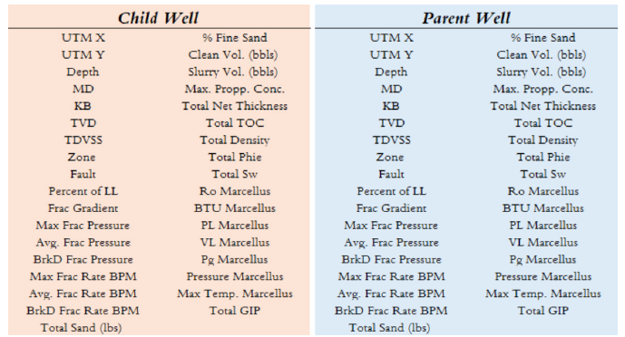
Figure 4:Distribution of distance between the child and parent well frac stages and percentage of Frac-Hit in each group.

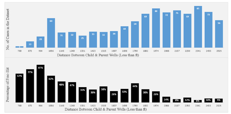
Figure 4 clearly implies that even though the number of frac stages has increased by distance, the percentage of Frac-Hit reduces drastically. In other words, by increasing the distance between the child and the parent well, probability of Frac-Hit reduces. For a better visualization, the 10 distance intervals were lumped to three intervals (less than 1,500 ft., between 1,500 to 2,000ft., and more than 2,000ft.). As shown in Figure 5, when the distance between the child and parent well is less than 1,500ft., more than half of frac stages (52%) caused a Frac-Hit. However, when the distance between the child and parent well is between 1,500 to 2,000ft., only 30% of frac stages showed Frac-Hit and finally the Frac-Hit occurrence drops to 8% when the distance between the child and parent well exceeds 2,000ft. It can be concluded that by increasing the distance between the child and parent wells, the chance of Frac-Hit reduces as the hydrocarbon recovery from the shale asset. Furthermore, the increase in the distance does not fully eliminate the chance of Frac-Hit and remains 8% at distances above 2,000ft. in this study. There are two more parameters used by operating companies, “On Plane” and “Shielded”, besides the distance between the child and parent wells in decision-makings to avoid Frac-Hit. The “On Plane” parameter specifies if the parent well is within the frac stage of the child well. The “Shielded” identifies if the parent well is protected by another producing well located between the parent and the child well.

Figure 5:Frac-Hit occurrence as a function of distance between the child and the parent well.

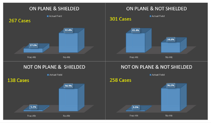
Putting the three parameters of Distance, On Plane and Shielded together would create a flowchart to predict if Frac-Hit happens or not. Based on this flowchart, shown in Figure 6, if the distance between the child and parent well is greater than a cut-off distance (XCD), no Frac-Hit will be predicted. However, if the distance is below the cut-off distance, then “On Plane” and “Shielded” parameters should be checked and only if the stages are “On Plane” and “not Shielded”, Frac-Hit will be predicted. In other words, Frac- Hit occurrence is predicted only under a specific scenario when the distance is below the cut-off, stages of the child and parent wells are “On Plane” and the parent well is “not Shielded” and any other possible scenario would predict no Frac-Hit. The flowchart can also be interpreted as a decision tree where the distance has the most importance in the decision-making and prediction (Frac-Hit or No Hit) and “On Plane” and “Shielded” status are the next orders of importance in the Frac-Hit occurrence prediction. The dataset was categorized into four groups based on their status of “On Plane” and “Shielded”. Figure 7 demonstrates this distribution and percentage of Frac-Hit occurrence in each category. Figure 7 clearly shows that the highest percentage of Frac-Hit (65.4%) occurred when parent wells were “On Plane” and not “Shielded” and the least percentage of Frac-Hit (3.5% and 5.1%) occurred when wells were not “On plane”. This actually aligns with the industry’s common practice that the highest chance of Fric-Hit occurrence is when the wells are “On Plane” and not “Shielded”. The problem arises when only 65.4% of the stages had Frac-Hit when they were “On Plane” and not “Shielded” while based on Figure 6 flowchart it should show 100% Frac-Hit!

Figure 6:Frac-Hit prediction decision tree.

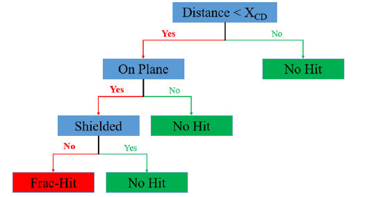
Figure 7:Frac-Hit occurrence distribution on the actual field data based on “On Plane” and “Shielded” parameters.

To evaluate the performance of the industry practice on the dataset, Figure 6 flowchart should be implemented on the data. Since the largest distance between the child and parent wells in the used dataset was 2,525ft., this distance was used as the cut-off distance (XCD). Choosing this cut-off distance would also provide the best possible performance for the common practice predictions. Figure 8 demonstrates the results of this implementation. According to Figure 8, 41% of frac stages (396 cases) were not “On Plane” and over all 16 cases out of 396 were misclassified as “No Hit” while they were actual Frac-Hits. In addition, there were 301 cases when wells were “On Plane” and not “Shielded”, 104 cases (34.5%) were misclassified as “No Hit”. Finally, in 267 cases when the wells were “On Plane” and “Shielded”, 47 cases were misclassified as Frac-Hit. In summary, 167 cases out of 964 cases (17.3%) were predicted wrong and the biggest contributor was when Frac-hit occurrence had the highest chance (“On Plane” and not “Shielded”). Figure 9 shows a comparison between the actual data and industry’s common practice prediction. To evaluate the performance of classification problems like Frac-Hit occurrence, which is a binary classification problem, confusion matrix is used. Confusion matrix is a specific table layout for summarizing the performance of a classification problem that provides four different combinations of predicted and actual values. Calculating the confusion matrix provides a better idea of what the classification model gets right and what types of errors it makes. Figure 10 shows the breakdown of the confusion matrix for a binary classification.

Figure 8:Industry practice prediction of Frac-Hit occurrence.

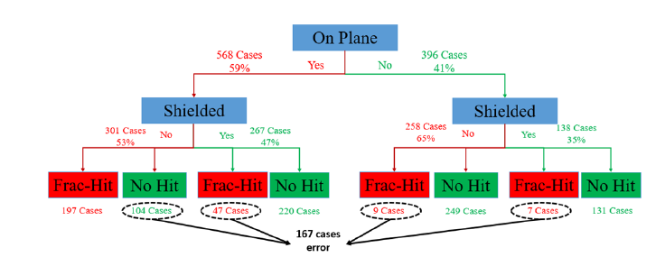
Figure 9:Comparison of Industry practice prediction of Frac-Hit with actual data.

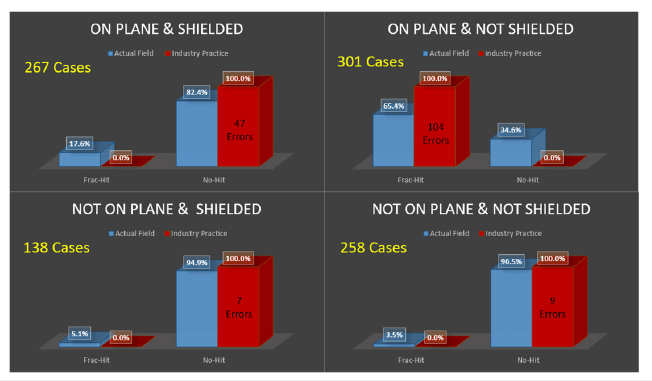
Figure 10:Confusion matrix components.

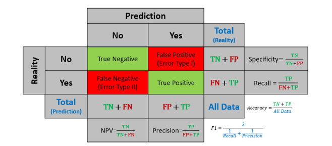
Confusion matrix table has a four main category layout:
A. True Negative: the predictive model classifies a negative outcome correctly.
B. False Positive: the predictive model classifies a negative outcome wrong, also called “Error Type I”.
C. False Negative: the predictive model classifies a positive outcome wrong, also called “Error Type II”.
D. True Positive: the predictive model classifies a positive outcome correctly.

The four main categories of confusion matrix also have some derivatives, which are used as metrics of model performance:
a) Recall: the ratio of Ture Positive to all positive conditions, also known as True Positive Rate (TPR)
b) Precision: the ratio of Ture Positive to all positive predicted outcomes.
c) Negative Predictive Value (NPV: the ratio of True Negative to all negative predicted outcomes.
d) Specificity: the ratio of Ture Negative to all negative conditions, known as True Negative Rate (TNR)
e) Accuracy: the ratio of total correct predictions to all the cases.
f) F1-Score: the harmonic average of Recall and Precision.

Among these six-performance metrics, Recall, Precision, Accuracy and F1-Score are the most popular ones. Recall is usually important when False Positives burden lower cost than False Negatives and objective is to lower the False Negatives. Precision is important when focus is on the True Positives. Accuracy is important when the dataset is symmetric in outcome classes and F1-Score is used when dataset is not symmetric. The confusion matrix was calculated for the industry practice model and presented in Figure 11. Figure 11 clearly shows that 104 cases of the False Positive cases, when the industry model predicts Frac-Hit while Frac-Hit did not happen in reality, has resulted in a low Precision value of 65%. The cost of low Precision can be reflected in the hydrocarbon recovery factor. On the other hand, 63 cases of False Negatives, when the industry model predicts no Frac-Hit while Frac-Hit occurs in reality, has resulted in a low Recall value of 75%. The cost of low Recall can be reflected in the increase of water production and the decrease of hydrocarbon production after Frac-Hit.

Figure 11:Confusion matrix for industry practice model.

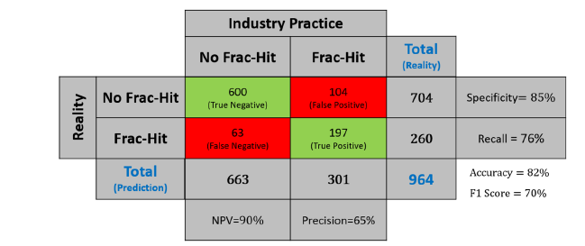
An ideal confusion matrix would have zero False Positive and zero False Negative cases resulting in Recall and Precision to be 100%. However, in practice there is always a trade-off between the four categories of True Negative, True Positive, False Negative and False Positive. If the objective is to minimize the False Positives, i.e., to increase the recovery factor, then Precision should be optimized. However, if the objective is to minimize the False Negatives, i.e., predicting Frac-Hit occurrence correctly, then Recall should be optimized. In this study, we tried to minimize both False Positives and False Negatives simultaneously (Increase both Recall and Precision simultaneously). To do so, F1-score should be optimized as the dataset was imbalanced with ratio of almost 1 to 3 between classes of Frac-Hit and no Frac-Hit. Snapshot modeling of Frac- Hits, which is a purely fact-based AI/ML technique incorporates many other field measurements besides distance, “On Plane” and “Shielded” parameters. These parameters include well characteristics, reservoir characteristics, completion and hydraulic fracturing design of both child and parent wells, as shown in Figure 3.

For the snapshot modeling of Frac-Hits, Artificial Neural Networks (ANN) model was implemented. For that, 964 frac stages in the dataset were divided into three categories of training, calibration and blind validation with proportions of 60%, 15% and 25%. The category of each frac stage was determined randomly. The training dataset was used for training the ANN, the calibration dataset also known as validation dataset was used for unbiased validation of the training dataset during the training process. The blind validation dataset, also known as test set, was the dataset that has not been used in the training process and provides an unbiased validation of the final model. In addition to hyperparameter tuning, a 5-fold cross-validation was also implemented during the training process to achieve a robust model. The architecture and details of the ANN after hyperparameter tuning are shown in Table 1. After training the ANN, the shale analytics model was used to predict the training and the blind validation datasets. Then the matrix confusion of each dataset was calculated. To have a fair comparison between the industry practice model and shale analytics one, the confusion matrix was also calculated for training and blind datasets based on the industry practice model. Figure 12 shows the comparison between industry practice and shale analytics models for the training datasets.

Table 1:ANN architecture.

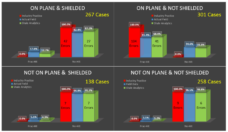
Figure 12 shows that Recall has improved from 75% to 84%, Precision has improved from 64% to 84%, and subsequently the Accuracy and F1-score have increased from 82% to 91% and 69% to 84%, respectively. Overall, the False Positive errors have reduced from 82 to 31 cases (72% less error) and False Negative errors have reduced from 49 to 31 cases (27% less error). Similar approach was implemented on the blind validation dataset and the confusion matrix for both techniques of industry and shale analytics were calculated and compared. As Figure 13 shows, similar to training dataset, all metrics of Recall, Precision, Accuracy and F1-score have significantly improved in the shale analytics. The overall comparison of the actual data with industry practice and shale model in Frac-Hit prediction using parameters of “On Plane” and “Shielded” parameters are shown in Figure 14.

Figure 12:Comparison between confusion matrices of industry practice and shale analytics models on the training dataset.

Figure 13:Comparison between confusion matrices of industry practice and shale analytics models on the blind validation dataset.

Figure 14:Comparison of actual Frac-Hits vs. the industry practice and shale analytics techniques.

Artificial intelligence and Machine Learning is pure datadriven, fact-based technology without assumptions, simplifications and interpretations. This technology can provide more realistic and accurate results in hydrocarbon recovery in shale assets.

1. Mohaghegh SD (2017) Shale analytics; data-driven analytics in unconventional resources. (1^st edn), Springer Nature, Springer International Publishing, Switzerland.
2. Mohaghegh SD (2017) Data-driven reservoir modeling. Society of Petroleum Engineers, Texas, USA.
3. Mohaghegh SD (2020) Frac-hit dynamic modeling using artificial intelligence & machine learning. Unconventional Resources Technology Conference, Austin, Texas, USA, pp. 4947.
4. Quintero G. (2022) Quantitative analysis of rate transient analysis in unconventional shale gas reservoirs. Master’s Thesis, Department of Petroleum & Natural Gas Engineering, West Virginia University.
5. Raterman KT, Farrell HE, Mora OS, Janssen AL, Gomez GA, et al. (2017) Sampling a stimulated rock volume: An eagle ford example. Unconventional Resources Technology Conference, Austin, Texas, USA.
6. Tyree R (2018) Predicting frac-hit using artificial intelligence; application in Marcellus shale. Master’s Thesis, Department of Petroleum & Natural Gas Engineering, West Virginia University.