Maximum Entropy Risk Model for Investment Management

Introduction

Every investor wants to maximize his profits by selecting proper strategy for investment. There are investments like government and bank securities, real estate, mutual funds and blue chips stocks, which have low return but are relatively safe because of a proven record of non-volatility in price fluctuations. On the other hand, there are investments which bring high returns, but may be prone to a great deal of risk and the investor makes loss in case the investment goes sour. To overcome the above mentioned problem the investor should invest his funds in a spread of low and high risk securities in such a way that the total expected return for all his investments is maximized and at the same time his risk of losing his capital is minimized. Since the various outcomes as well as the probabilities of these outcomes and the return on a unit amount invested in each security are known, therefore, there is not much difficulty in maximizing the expected return. However, the main problem is to overcome risk factor. The earliest measure proposed regarding risk factor was variance of returns on all investments in the portfolio and was based on the argument that risk increases with variance. Markowitz [1] gave the concept of mean-variance efficient frontier and this enabled him to find all the efficient portfolios that maximize the expected returns and minimize the variance. Kapur and Kesavan [2] made a brief account of application of entropy optimization principles in minimizing risk in portfolio analysis. Hooda and Kapur [3] have applied these principles in characterizing crop area distributions for optimal yield.

Markowitz Mean-Variance-Efficient Frontier

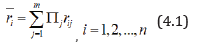
Let πj be the probability of jth outcome for j=1,2,…,m and r_ij be the return on ith security for i=1,2,…n, when jth outcome occurs.

Then the expected return on the ith security is

Variance and covariance of returns are given by

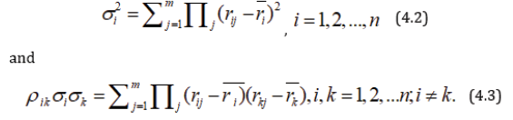
and

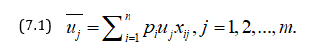
A person decides to invest proportions x₁, x₂,…, x_n of his capitals in n securities. if x_i≥0 for all i and x_i=1, then the mean and variance of the expected returns are given by

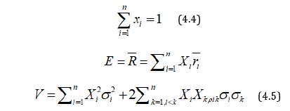
Markowitz suggested that x₁, x₂,…, x_n be chosen to maximize E and to minimize V or alternatively, to minimize V keeping E at a fixed value.

Now

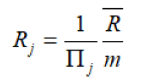
Where, i.e. R_j is the return on investment when jth outcome arises, and  is the mean return on investment.

Figure 1:

Corresponding to each vector (x₁, x₂,…, x_n), there are certain values of E and V, so that corresponding to each portfolio, there is unique point in the E-V plane. In the (Figure 1) the arc AB gives the lower boundary at the convex region obtained. In this figure it can be easily seen that the portfolio corresponding to P is more efficient than the portfolio corresponding to Q because the mean return for both is the same, but variance for Q is greater than that of P. Similarly, the portfolio corresponding to P is also more efficient than the portfolio corresponding to R, because in both cases the variance is equal, while the mean return for P is higher than that for R. Thus the portfolio corresponding to any other point on the arc AB is more efficient than a portfolio corresponding to any other point inside the convex region. However, portfolios corresponding to different points on the arc AB are not comparable, because in one portfolio the mean return may be higher; while for the other variance may be smaller. The portfolio corresponding to points of the arc AB are called mean-variance efficient frontier. If a person chooses the portfolio corresponding to B it gives the highest possible value for E, but V is large at B. This means the person is interested in making his expected income large and does not mind whether variance becomes large and his risk is increased. Such persons who do not worry about risks are also known as risk-prone. On the other hand, persons who want to avoid risk and are cautious are called risk-averse and they will choose points near A. Thus, the choice of point on the arc AB depends on the attitude to the risk of the investor concerned.

Entropy Mean-Variance Frontier

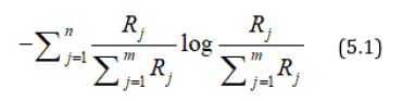
One of the investor’s objective is to diversify his portfolio so that out of all points on the mean-variance efficient frontier, he chooses that portfolio for which his investments in different stocks as equal as possible i.e. to make R₁, R₂,….., R_m as equal as possible among themselves. Any departure of R₁, R₂,….., R_m from equality is considered a measure of risk which can be minimized if we choose R₁, R₂,….., R_m so as to maximize the entropy measure

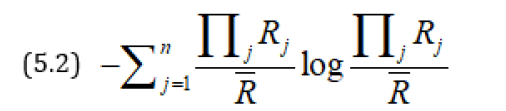
Since this does not include πj’s, therefore, we can modify the principle to say that πjRj’s should be as equal as possible i.e. the entropy of the probability distribution should be as large as possible. For this we maximize

Subject to

Applying Lagrange’s method of multipliers, we get

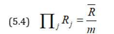
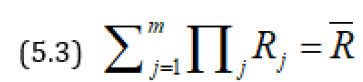
Thus according to our first principle RJ = , while according to

second principle

 If i.e. if the outcomes are equally likely, the two principles give the same results.

Again since we want R_j’s to be as equal as possible we want the probability distribution to be as close to the probability distribution as possible. So, we chose x₁, x₂,…, x_n to minimize either D(P_j, π_j) or D(π_j, P_j). If we use Kullback and Leibler [4]’s measure, then we have

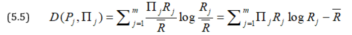
Since log is constant, therefore, it implies that should be as small as possible. This is the third principle. Next to minimize D(π_j, P_j) we again apply Kullback-Leibler’s measure and get

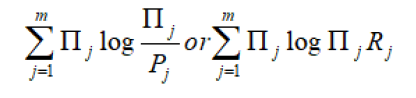
should be as small as possible, which is fourth principle. We can also use Harvda and Charvat [5] measure of directed divergence or cross-entropy. In that case we have to minimize

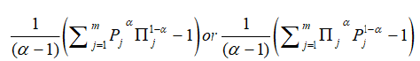
Thus according to 5^th and 6^th principle, we choose x₁, x₂,…, x_n to minimize respectively

Risk Aversion Index

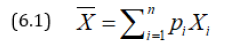
Let us consider a lottery in which the returns are x₁, x₂,…, x_n with probabilities p₁, p₂,…, p_n so that mean monetary return is

It may be noted that the utility of an amount x is not always proportional to x. If the monetary value is doubled, for some persons the utility increases, but it is less than double of the previous one. Such persons are also called risk-averse and those for which the utility is more than doubled will be called risk-prone. Thus, the attitude to risk of every person is characterized by u(x). For risk-averse persons u(x) increases at a decreasing rate i.e. u’(x)<0 or u(x) is concave function, while for risk-prone persons u’(x)>0 and (x) is a convex function and for risk-neutral persons u’(x)=0. Pratt [6] and Arrow [7] defined a risk-aversion index (RAI) as

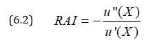
It can be easily verified that if u(x)=log x, then RAI=1/x>0 and if u(x) = e^x, then RAI = 1/x<0 and RAI = 0 in case u(x)=x.

Next, we explain how the expression (4.2) can be obtained.

We define 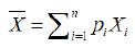  as certain monetary equivalent (CME) and define ~x by

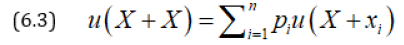
where X is the positive initial capital. (4.3) can be written as

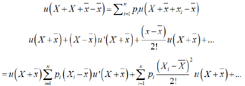
Neglecting  and higher orders, we have

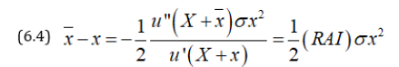
Thus, CME exceeds ~x by an amount proportional to RAI and this arises due to the attitude to risk of the investor. The concept of RAI can be generalized for u (x, y) and we get

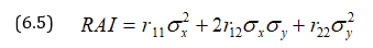
where risk averse functions are

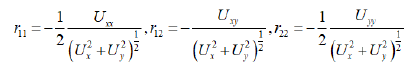
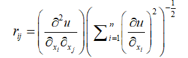
This can be further generalized for u (x₁, x₂,…, x_n) to get

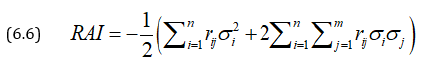
Where

If risk aversion index for two variables is 0, then    

which is an elliptic partial differential equation of second order.

Pareto Optimal Sharing of Risks

A number m of persons agrees to share risks in a business on basis of optimal sharing of risks and profits in such a manner that no individual can increase his expected utility without decreasing the expected utilities of others. Let a risk have n possible states s₁, s₂,…, s_n with payments x₁, x₂,…, x_n and with probabilities p₁, p₂,…, p_n. Let payments be partitioned among m individuals whose utility functions are u₁, u₂,…, u_m. Let xij be the payment of jth individual in case of ith outcome, then the expected utility of this partitioned risk is given by

where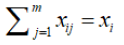

We can plot the m expected utilities in m dimensional space. If the m expected utilities are negative, then no partition is acceptable because (0, 0,…,0) will be preferred by all. In case all u_i’s are positive, we maximize

Thus, we get a linear hyperplane

The envelope of this hyperplane gives the equation of the Pareto optimal hyperplane. All points of this hyper-surface are accepted but which point is chosen depends on the relative bargaining power of the partner or they can choose the point of intersection with the line .

Thus, this equitable Pareto optimal sharing can be obtained instead of individual. We can have groups fighting for increasing their social, political or economic utilities and arriving at Pareto Optimal Equilibria. When these equilibria are disturbed, new Pareto optimal equilibrium positions have to be obtained.

Maximum Entropy Principle in Risk Sharing

The Pareto optimal boundary gives infinity of solutions and we need one more criterion to get a unique solution. This is possible by considering that payments are divided as uniformly as possible subject to other constraints. For this Kapur [8] suggested to maximize the following measure of entropy:

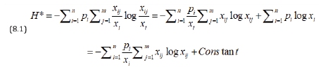
Thus out of all Pareto Optimal solutions we choose that one which maximizes H*.

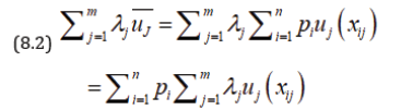
Raiffa [9] has shown that the Pareto Optimal solution can be obtained by maximizing

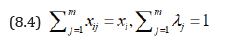
subject to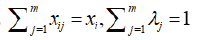

This will determine in term of

Since therefore, H* is function of

We choose satisfying for

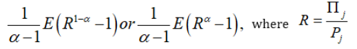
i. Special case of exponential utility function

Let us consider

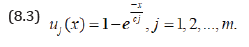
we maximize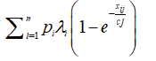

subject to,

Following Lagrange’s method of multiplier, we get

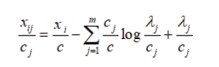
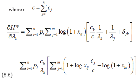
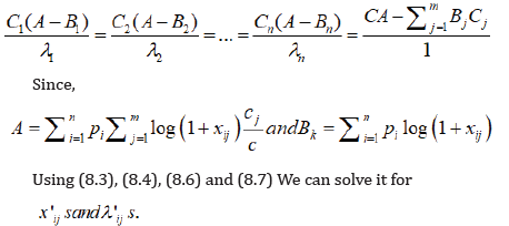
Substituting in (6.1) and differentiating w.r.t. k, we have (8.7)

References

1. Markowitz HM (1959) Portfolio selection: efficient diversification of investments. (2^nd edn), John Wiley, New York, USA.
2. Kapur JN, HK Kesavan (1992) Entropy optimization principles with applications. Academic Press, USA pp. 3-20.
3. Hooda, DS and JN Kapur (2001) Crop area distributions for optimal yield. OP Search 38: 407-418.
4. Kullback S , RA Leibler (1951) On information and sufficiency. Ann Math Stat 22(1): 79-86.
5. Harvda J, F Charvat (1967) Quantification method of classification processes-concept of α-entropy. Kybernetika 3: 30-35.
6. Pratt JW (1964) Risk aversion in the small and in the large. Econometrics 32(1/2): 122-136.
7. Arrow KJ (1971) Essays on the theory of risk bearing. Markhan Publishers, Chicago, USA.
8. Kapur JN (1989) Maximum entropy models in science and engineering. Wiley Eastern Limited, New Delhi, India.
9. Raiffa H (1968) Decision analysis. Addison Wesley, USA.

© 2020 Prabuddha Gupta. This is an open access article distributed under the terms of the Creative Commons Attribution License , which permits unrestricted use, distribution, and build upon your work non-commercially.