
- About Us
- Information
-

The Author ensures that the research has been conducted responsibly and ethically with adherence to all relevant regulations. read more..
- For Authors
- For Reviewer
- Manuscript Guidelines
- Membership
- Publication Ethics
-
- Journals
- Reprints
- e-Books
- Videos
- Policies
- Contact Us
 COVID-19
- Submissions


Full Text
Open Access Biostatistics & Bioinformatics
Breast Cancer Prediction Using Bayesian Logistic Regression
Michael Chang1, Rohan J Dalpatadu1, Dieudonne Phanord1 and Ashok K Singh2*
1 Department of Mathematical Sciences, University of Nevada, USA
2 William F Harrah College of Hotel Administration, University of Nevada, USA
*Corresponding author:Ashok K Singh, William F Harrah College of Hotel Administration, University of Nevada, Las Vegas, USA
Submission: July 26, 2018;Published: September 25, 2018

ISSN: 2578-0247 Volume2 Issue3
Abstract
Prediction of breast cancer based upon several features computed for each subject is a binary classification problem. Several discriminant methods exist for this problem, some of the commonly used methods are: Decision Trees, Random Forest, Neural Network, Support Vector Machine (SVM), and Logistic Regression (LR). Except for Logistic Regression, the other listed methods are predictive in nature; LR yields an explanatory model that can also be used for prediction, and for this reason it is commonly used in many disciplines including clinical research. In this article, we demonstrate the method of Bayesian LR to predict breast cancer using the Wisconsin Diagnosis Breast Cancer (WDBC) data set available at the UCI Machine Learning Repository.
Introduction
Figure 1:Estimated number of new cases in US for selected cancers-2018.

Cancer is a group of diseases characterized by the uncontrolled growth and spread of abnormal cells [1]. Globally, breast cancer is the most frequently diagnosed cancer and the leading cause of cancer death among females, accounting for 23% of the total cancer cases and 14% of the cancer deaths [2]. In US as well, breast cancer is the most frequent type of cancer (Figure 1). Bozorgi et al. [3] used logistic regression for the prediction of breast cancer survivability using the SEER (Surveillance, Epidemiology, and End Results) database NCI (2016) of 338,596 breast cancer patients. Salama et al. [4] compared different classifiers (decision tree, Multi-Layer Perception, Naive Bayes, Sequential Minimal Optimization, and K-Nearest neighbor) on three different data sets of breast cancer and found a hybrid of the four methods to be the best classifier. Delen et al. [5] used artificial neural networks (ANN), decision trees (DT) and logistic regression (LR) to predict breast cancer survivability using a dataset of over 200,000 cases, using 10-fold cross-validation for performance comparison. The overall accuracies of the three methods turned out to be 93.6%(ANN), 91.2%(DT), and 89.2%(LR). Peretti & Amenta [6] used logistic regression to predict breast cancer tumor on a data set with 569 cases and obtained overall accuracy of 85%. Barco et al. [7] used LR on a data set of 1254 breast cancer patients to predict high tumour burden (HTB), as defined by the presence of three or more involved nodes with macro-metastasis. Three predictors (tumour size, lymphovascular invasion and histological grade) were found to be statistically significant. LR and ANN are commonly used in many medical data classification tasks. Dreiseitl & Ohno-Machado [8] summarize the differences and similarities of these models and compare them with a few other machine learning algorithms. Van Domelen et al. [9] estimated the LR model from a Bayesian approach when the predictors are known to have errors. In a study to determine the main causes of complications after rad- ical cystectomy [10], multivariate logistic regression was used to show that the main causes of complications were anemia before surgery, weight loss, intraoperative blood loss, intra-abdominal infection. In the present article, we use the Wisconsin Diagnostic Breast Cancer Data Set of 569 observations on 32 variables [11] to predict breast cancer using the method of Bayesian LR. We provide a description of the Bayesian LR in the next section.
Bayesian Estimation of Logistic Regression Model
The Logistic Regression (LR) model is a special type of regression model fitted to a binary (0-1) response variable Y, which relates the probability that Y equals 1 to a set of predictor variables:
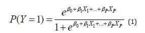
where X1, …, XP are P predictors, which can be continuous or discrete. The above model can be expressed in terms of log-odds as follows [12] :

In the frequentist approach, given the random sample,
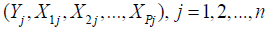
Yj are n independent realizations of a Bernoulli experiment with probability of success P(Yj=1) given by (1); the model coefficients βj are unknown constants to be estimated from data. The likelihood function of the sample is
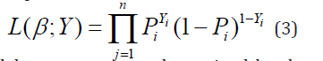
The LR model parameters are determined by the method of maximum likelihood estimation (MLE), which finds the β-coefficients that maximize the logarithm of the likelihood function

In the Bayesian approach, the model coefficients (β1, β2, …,βP) are realizations of a P-variate random vector generated from the joint prior distribution; any prior knowledge about the β-coefficients can be incorporated in this joint prior distribution. All inferences drawn using Bayesian approach are conditional on data, and large sample theory of estimates is not needed. The conditional sample likelihood given by expression (3) is combined with the joint prior distribution of the parameters via the Bayes theorem [13] to obtain the joint posterior distribution of the model parameters, as shown below.
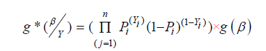
“where g*”(β ̱|Y ̱)” is the joint posterior distribution”,” and “ g(β ̱)” the joint posterior distribution”
“of the parameters “ β ̱. If very little prior knowledge exists about the model parameters, we can use a vague prior. The marginal posterior distributions are numerically computed from the joint posterior distribution, and the means of these distributions are the parameter estimates. We can also obtain 95% confidence intervals of the parameters from these marginal posterior distributions. In Bayesian framework, these confidence intervals are called credible sets. In computing a credible set, it is desirable to obtain a credible set with shortest interval. The 95% highest posterior density (HPD) credible set contains only those points with largest posterior probability distribution [14]. A comparison of Bayesian and Frequentist approaches for estimation of predictive models is provided in [15- 18].
Performance Measures for Prediction of a Binary Response
A large number of performance measures for multi-level classifiers exist in machine learning literature [19]. Commonly used performance measures of classifiers are accuracy, precision, recall and the geometric mean F1 of precision and recall [20,21]. To compute these measures, we first need to calculate the 2x2 confusion matrix in Table 1 The performance measures accuracy, precision, recall and F1 are calculated for each category 0 and 1 from the following formulas :
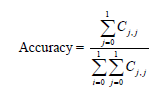
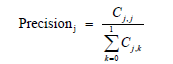
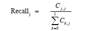
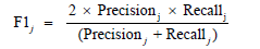
j = 0,1
Table 1:

Bayesian Prediction of Breast Cancer
The data set used here is the Wisconsin Diagnostic Breast Cancer (WDBC) Data Set, which is well-known in Machine Learning literature [9]. This data set has 569 observations on 32 variables including the binary response variable “Diagnosis” which takes values M (malignant) and B (benign). There are 10 features are computed for each cell nucleus:
1. Radius (average distance from center to points on the perimeter).
2. Texture (standard deviation of gray-scale values).
3. Perimeter.
4. Area.
5. Smoothness (local variation in radius lengths).
6. Compactness (perimeter^2 / area - 1.0).
7. Concavity (severity of concave portions of the contour).
8. Concave points (number of concave portions of the contour).
9. Symmetry.
10. Fractal dimension (“coastline approximation” - 1).
The mean, standard error, and “worst” or largest (mean of the three largest values) of these features were computed for each image, resulting in a total of 30 features for each of the 569 patients. Detailed descriptions of how these features are computed can be found in [22,23]. Since 20 of the 30 predictors were computed from data, high multicollinearity is expected in this data set. This can be seen in Figure 2, which is a plot of the correlations among the predictors in the WDBC data set.
Figure 2:Correlation plot of 30 predictors in WDBC data set.

There are three common approaches for fitting a LR model when high multicollinearity exists in the data. Aguilera et al. [24] used Principal Components Analysis (PCA) to obtain independent predictors (Principal Components) and then used LR; simulated data was used in this study. Asar [25] proposed shrinkage type estimators for fitting LR models and used Monte Carlo simulation experiments to show that the shrinkage estimators perform better than the standard MLE estimator. Another simpler and more common approach is to drop predictors with high variance inflation factor (VIF) values and obtain a model in which largest VIF is 5 [26]. This is the approach taken in this article.
Result for WDBC Data Set
All of the analyses presented here are performed using the statistical software environment R [27]. The WDBC data set of 569 cases was first split into a 75% training set of 427 observations and 25% test set of 142 observations. The LR Model for the training set, with all 30 predictors in the model had VIF falling in the range 78 to 123630, with none of the predictors significant (Table 2); this is due to extremely high multicollinearities among the 30 predictors. After eliminating predictors with VIF>5 one by one, the final LR model was obtained (Table 3) with Texture, Area, Concavity, and Symmetry in the model. A comparison of Table 2 & 3 shows how multicollinearities affect the estimation of LR model coefficients:
1. In the LR model with all predictors, all P-values are 1 i.e., none of the predictors are significant.
2. The estimated coefficients of the final predictors in the LR model with all predictors are all negative, when these coefficients should all be positive.
3. The standard errors (SE) of the final predictors in the LR model with all predictors are orders of magnitude higher than the corresponding estimates.
4. The final LR model, which has Texture, Area, Concavity, and Symmetry as the significant predictors, does not suffer from any of the above three issues; each coefficient is positive as it should be, and each predictor is highly significant.
Table 2:Bayesian LR model with all 30 predictors in the model fitted to the training set

Note: VIF values for LR model with all predictors in are very high: minimum(VIF)=78, max(VIF)=123630.
Figure 3:Posterior distributions of bayes estimates of logistic regression model coefficients and their 95% HPD credible sets.

Figure 3 shows the posterior distributions and the 95% HPD credible sets for the coefficients of the predictors in the final LR model; the 95% HPD credible sets are: βTexture: (0.16, 0.37), βArea: (0.008, 0.016), βConcavity: (16.65, 36.30), βArea: (3.22, 40.28). Observe that all four 95% HPD credible sets fall to the right of 0. The final LR model was next used to predict response “Diagnosis” for both the training and test data sets. The confusion matrices and overall accuracies for the training and test sets are shown in Table 4 & 5. The values of precision, recall and F1 measures for both training and test data are all quite high, as shown in Table 6.
Table 3:Final Bayesian LR model fitted to the training set.

Note: Each of the four VIF values is < 5
Table 4:Training set. Overall accuracy for the training set=93.2%.

Table 5:Test set. Overall accuracy for the test set=93.0%.

Table 6:

References
- https://www.cancer.org/content/dam/cancer-org/research/cancerfacts- and-statistics/annual-cancer-facts-and-figures/2018/cancerfacts- and-figures-2018.pdf
- Jemal A, Bray F, Center MM, Ferlay F, Ward E, et al. (2011) Global Cancer Statistics. CA Cancer J Clin 61(2): 69-90.
- Bozorgi M, Taghva K, Singh A (2017) Cancer Survivability with Logistic Regression. 2017 Computing Conference 2017, London, UK.
- Salama GI, Abdelhalim MB, Zeid MA (2012) Breast Cancer diagnosis on three different datasets using multi-classifiers. International Journal of Computer and Information Technology 1(1): 36-43.
- Delen D, Walker G, Kadam A (2004) Predicting breast cancer survivability: a comparison of three data mining methods. Artif Intell Med 34(2): 113-27.
- Peretti A, Amenta F (2016) Breast cancer prediction by logistic regression with CUDA parallel programming support. Breast Can Curr Res 1(3): 111.
- Barco I, García Font M, García Fernández A, Giménez N, Fraile M, et al. (2017) A logistic regression model predicting high axillary tumour burden in early breast cancer patients. Clin Transl Oncol 19(11): 1393- 1399.
- Dreiseitl S, Ohno Machado L (2002) Logistic regression and artificial neural network classification models: a methodology review. Journal of Biomedical Informatics 35(5-6): 352-359.
- Van Domelen DR, Mitchell EM, Perkins NJ, Schisterman EF, Manatunga AK, et al. (2018) Logistic regression with a continuous exposure measured inpools and subject to errors. Statistics in Medicine, pp. 1-15.
- Atduev V, Gasrataliev V, Ledyaev D, Belsky V, Lyubarskaya Y, et al. (2018) Predictors of 30-day complications after radical Cystectomy. Exp Tech Urol Nephrol 1(3): ETUN.000514.
- Dua D, Karra Taniskidou E (2017) UCI Machine Learning Repository. University of California, School of Information and Computer Science, Irvine, USA.
- David GK, DG, Klein M (2010) Logistic Regression-A Self‐Learning Text, (3rd edn), pp. 7-9.
- Kruschke J (2015) Doing Bayesian Data Analysis, Elsevier, USA, pp. 87- 90.
- Rohan Dalpatadu, Gewali L, Singh AK (2002) Computing the Bayesian highest posterior density credible sets for the lognormal mean. International Conference on Environmetrics and Chemometrics 13(5- 6): 465-472.
- Newcombe PJ, Reck BH, Sun J, Platek GT, Verzilli C, et al. (2012) A comparison of Bayesian and frequentist approaches to incorporating external information for the prediction of prostate cancer risk. Genet Epidemiol 36(1): 71-83.
- Paul GA, Jeffrey PH, Sujata MB, Christopher MR, Evelyn JE, et al. (2012) Frequentist and Bayesian Pharmacometric-Based Approaches To Facilitate Critically Needed New Antibiotic Development: Overcoming Lies, Damn Lies, and Statistics. Antimicrob Agents Chemother 56(3): 1466-1470.
- Peter A, David NC, Jack V Tu (2014) A comparison of a Bayesian vs. a frequentist method for profiling hospital performance. The Open Epidemiology Journal 7(1): 35-45.
- Wioletta G (2015) The advantages of Bayesian methods over classical methods in the context of credible intervals. Information Systems in Management 4(1): 53-63.
- Sokolova M, Lapalme G (2009) A systematic analysis of performance measures for classification tasks. Information Processing and Management 45(4): 427-437.
- James G, Witten D, Hastie T, Tibshirani R (2013) An introduction to statistical learning. Springer, New York, USA.
- Guillet F, Hamilton H (2007) Quality measures in data mining. Springer, New York, USA.
- Street WN, Wolberg WH, Mangasarian OL (1991) Nuclear feature extraction for breast tumor diagnosis. International Symposium on Electronic Imaging: Science and Technology 1905: 861-870.
- Wolberg WH, Street WN, Mangasarian OL (1994) Machine learning techniques to diagnose breast cancer from image-processed nuclear features of fine needle aspirates. Cancer Letters 77(2-3): 163-171.
- Ana MA, Manuel E, Mariano JV (2006) Using principal components for estimating logistic regression with high-dimensional multicollinear data. Computational Statistics & Data, Analysis 50(8): 1905-1924.
- Yasin A (2017) Some new methods to solve multicollinearity in logistic regression. Communications in statistics - simulation and computation 46(4): 2576-2586.
- Montgomery DC, Peck EA, Vining GG (2001) Introduction to linear regression analysis, (3rd edn), Wiley, New York, USA.
- R Core Team (2017) R: A language and environment for statistical computing. R Foundation for Statistical Computing, Vienna, Austria.
© 2018 Ashok K Singh. This is an open access article distributed under the terms of the Creative Commons Attribution License , which permits unrestricted use, distribution, and build upon your work non-commercially.
Editor In Chief


.jpg)


Signup for Newsletter

Quick Links
 Editorial Board Registrations
 Submit your Article
 Refer a Friend
 Advertise With Us
Our Recent Edition

.jpg)


Top Editors


.jpg)


.bmp)
.jpg)
.png)
.jpg)


.jpg)


.png)

.png)


.png)


Financial Support

Sponsors

Latest e-Books

Latest Video

 a Creative Commons Attribution 4.0 International License. Based on a work at www.crimsonpublishers.com.
Best viewed in
a Creative Commons Attribution 4.0 International License. Based on a work at www.crimsonpublishers.com.
Best viewed in