The Optimum Selection of Imperfect Quality Economic Manufacturing Quantity and Process Mean

Introduction

Traditional Economic Manufacturing Quantity (EMQ) model is assumed implicitly that items produced are of perfect quality. However, product quality is not always perfect and is usually a function of the production process. Springer [1] provided the method of determining the most economic position of a process mean. Bisgaard et al. [2] presented an economic analysis for the problem of selecting the most favourable quality distribution for an industrial process. An important special case is that of selecting the best mean (target) value. The analysis, which takes into account the stochastic nature of the process, was illustrated by considering the problem of choosing the optimal amount of overfill in a filing operation. Rosenblatt & Lee [3] studied the effects of an imperfect production process on the optimal production cycle time. The system was assumed to deteriorate during the production process and produce some proportion of defective items. The optimal production cycle was derived and was shown to be shorter than that of the classical Economic Manufacturing Quantity model. The analysis was extended to the case where the defective rate is a function of the set-up cost, for which the setup cost level and the production cycle time are jointly optimized. They considered the case where the deterioration process is dynamic in its nature, i.e. the proportion of defective items is not constant. Both linear, exponential, and multi-state deteriorating processes were studied in their paper. Rahim & Banerjee [4] considered the problem of selecting the optimal production run for a process with random linear drift. A cost function per unit of finished product was derived. A search algorithm as well as a graphical method were suggested to find the optimal production run. They showed numerical examples of how to determine the optimal production run. They also performed a sensitivity analysis of the model. Carlsson [5] showed that the economic impact of the choice of process level for an industrial process depends on both internal and external conditions. Arcelus & Rahim [6] presented an economic model which incorporates the joint control of both variable and attribute quality characteristics of a product. Their objective was to simultaneously select the appropriate target values for the characteristics, so as to maximize the expected income per lot. Optimality conditions were derived for various probability distributions of the number of defects in a lot and computational experience were reported. Chen & Chung [7] considered the problem of joint determination of the optimal process mean and the production run for a process. It extended the quality selection process problem to production systems in which the process mean (target) shifts to an out-of-control state due to an assignable cause. Rahim & Tuffaha [8] incorporated the quality cost by introducing a Taguchi loss function for determining simultaneously the optimal process mean and production run. Rahim & Khan [9] presented a generalized model for the optimal determination of a production run and the initial settings of the process mean and process variance for a deteriorating production process. It is assumed that the process deteriorates due to tool wear-out. The probability that the process deterioration starts at a random point in times followed an exponential distribution. Quality loss from the target values was measured using Taguchi’s [10] quadratic loss function. The modified EMQ model with imperfect rework including the set-up cost, the holding cost, and the production cost is developed.

Economic Manufacturing Quantity Model

The following assumptions are made in order to develop an EMQ model: a) The manufacturing system consists of a single process or machine engaged in the production of a single item.
b) Quality of the product is perfect.
c) There is no shortage cost.
d) Demand of the product should be continuous i.e. production rate is always greater than demand rate (production rate > Demand rate).
e) The price per unit material in production is fixed. Purchasing quantity doesn’t change the price.
f) The total inventory cost of EMQ model includes the set-up cost and the holding cost, that is given by,

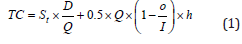
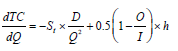
By differentiating TC with respect to Q, we have:

The second derivative of TC with respect to Q is,

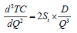
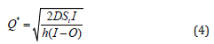
Equation (3) is positive. Hence by setting the first derivative of TC equal to zero. And finding the solution for Q, the optimum economic manufacturing quantity is:

Modified EMQ Model and Solution Procedure

The problem of EMQ model with imperfect quality was considered. A product will be inspected to check whether if it has been accepted, scrapped or sent to rework after the production process. Let y denote the normal quality characteristic of the product, the L₂ denote the Lower Specification Limit (LSL) of the product and the L₁ denote the Upper Specification (USL) of the product. A product will be accepted if L₂ y L₁, the product will be scrapped if y L₂, and the product will be sent to rework if yL1. The conforming units are shipped to consumers by the producers. For the rework process, the perfect and imperfect cases are considered. For the perfect rework, the product is reworked only once and the product of product of rework will be conformance. For the imperfect rework, the product may be reworked more than once, and the quality characteristics of rework are the same as that of production. The quality loss of conformance will be measured by Taguchi’s quadratics quality loss function. The following two modified EMQ model with the perfect and imperfect rework was considered./p>

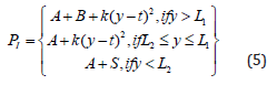
EMQ Model with Perfect Rework

It is assumed that the quality characteristic of product is normally distributed with unknown μ and the known standard deviation σ. sIn the perfect rework, the product is reworked only once, and the product of the rework will be conformance. The product quality of rework is distributed normally. Hence, the cost function of product with perfect rework is.

Hence, the expected cost of a product is,

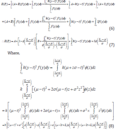
The probability of the product shipped to the customers is given by

Hence, thes modified EMQ model with perfect rework including the set-up cost, the holding cost, and the production cost is:

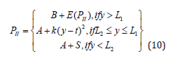
EMQ Model with Imperfect Rework

In the imperfect rework, the product may be reworked more than once, and the quality characteristic of rework is same as that of production. Hence, the cost function of product with imperfect rework is,

Hence, the expected cost of a product is,

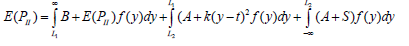
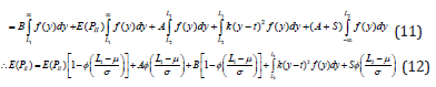
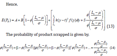
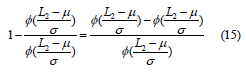
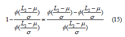
Therefore, the probability of the product that are shipped to customers are calculated by,

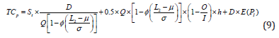
The modified EMQ model with imperfect rework including the set-up cost, the holding cost, and the production cost is,

It is difficult to show a closed form solution for the modified model (9) or (16) because the total inventory cost includes . For the given parameters, one can adopt the pattern search method for obtaining the optimum combination (Q*,μ*) of the above modified model (9) or (16).

Numerical Example

Let I=100?
O=80
S_t=20
h=1
A=0.2
B=2
S=1
L₂=10
L₁=15
t=12.5
D=2000
k=2/ (2.5 x 2.5)=0.32
σ=1.3

By solving the modified model (9), we have the optimum combination (Q*,μ*)=(657,12.32) with TC_p=1464.571 for the perfect rework product. By solving the modified model (16), we have the optimum combination (Q*,μ*)=(653,12.43) with TCI=1508.472 for the imperfect rework of product (Tables 1-5). The tables and figures below show the effect of parameter of the optimum solution for both modified models (Figures 1-10).

Table 1:close all
clear all
clc
x=[1600 1700 1800 1900 2000 2100 2200 2300 2400 2500 ].
Qp=[588 606 624 640 657 673 689 705 720 735].
Qi=[584 602 619 636 653 668 684 700 714 729].
tcp=[1183.601 1253.987 1324.272 1394.465 1464.571 1534.599 1604.553 1674.439 1744.26 1814.022].
tci=[1218.721 1291.302 1363.782 1436.17 1508.472 1580.694 1652.843 1724.924 1796.94 1868.897].

Table 2:close all
clear all
clc
x=[0.7 0.8 0.9 1 1.1 1.2 1.3 1.4 1.5 1.6].
Qp=[632 633 634 637 641 648 657 669 685 703].
Qi=[632 633 634 636 640 646 653 660 670 679].
tcp=[839.59 933.313 1035.416 1142.625 1251.669 1359.708 1464.571 1564.656 1658.905 1746.707].
tci=[839.717 934.061 1038.025 1149.428 1266.099 1386.261 1508.472 1631.623 1754.889 1877.61].
meanp=[12.5 12.49 12.48 12.46 12.42 12.38 12.32 12.25 12.17 12.08].
meani=[12.5 12.5 12.49 12.48 12.46 12.44 12.43 12.41 12.39 12.38].

Table 3:clear all
clc
x=[0.16 0.24 0.32 0.4 0.48 0.56 0.64 0.72 0.8].
Qp=[652 655 657 659 659 660 661 661 662].
Qi=[648 651 653 654 655 654 655 656 656].
tcp=[1029.295 1248.16 1464.571 1679.714 1894.125 2108.04 2321.626 2534.978 2748.156].
tci=[1051.81 1281.418 1508.471 1734.209 1959.174 2183.672 2407.814 2631.73 2855.478].
meanp=[12.45 12.37 12.32 12.29 12.27 12.25 12.23 12.22 12.21].
meani=[12.55 12.47 12.43 12.39 12.37 12.36 12.34 12.33 12.32].

Table 4:close all
clear all
clc
x=[85 90 95 100 105 110 115 120 125].
Qp=[1210 882 740 657 602 563 533 509 490].
Qi=[1202 875 734 653 598 559 529 505 486].
tcp=[1406.68 1432.361 1450.471 1464.571 1476.093 1485.79 1494.118 1501.38 1507.786].
tci=[1450.58 1476.261 1494.371 1508.471 1519.993 1529.69 1538.018 1545.28 1551.686].

Table 5:close all
clear all
clc
x=[60 65 70 75 80 85 90 95].
Qp=[465 497 537 588 657 758 929 1313].
Qi=[461 493 533 585 653 753 922 1303].
tcp=[1516.966 1505.412 1493.204 1479.502 1464.571 1447.625 1427.523 1401.326].
tci=[1560.866 1549.312 1536.9 1523.402 1508.471 1491.525 1471.423 1445.226].

Figure 1: plot (x,Qp,’-*r’)
hold on
plot (x,Qi, ‘-ok’)
xlabel (‘Demand Quantity’)
ylabel (‘Economic Manufacturing Quantity’)
legend (‘Qp’,’Qi’)

Figure 2: plot (x,tcp,’-*r’)
hold on
plot (x,tci, ‘-ok’)
xlabel (‘Demand Quantity’)
ylabel (‘Total Inventory Cost’)
legend (‘TCp’,’TCi’)

Figure 3: plot (x,Qp,’-*r’)
hold on
plot (x,Qi, ‘-ok’)
xlabel (‘Process Standard Deviation’)
ylabel (‘Economic Manufacturing Quantity’)
legend (‘Qp’,’Qi’)

Figure 4:plot (x,tcp,’-*r’)
hold on
plot (x,tci, ‘-ok’)
xlabel (‘Proces Standard Deviation’)
ylabel (‘Total Inventory Cost’)
legend (‘TCp’,’TCi’)

Figure 5:plot (x,meanp,’-*r’)
hold on
plot (x,meani, ‘-ok’)
xlabel (‘Process Standard Deviation’)
ylabel (‘Mean’)
legend (‘Mean(Perfect)’,’Mean(Imperfect)’)

Figure 6:plot (x,Qp,’-*r’)
hold on
plot (x,Qi, ‘-ok’)
xlabel (‘Quality Loss Coefficient’)
ylabel (‘Economic Manufacturing Quantity’)
legend (‘Qp’,’Qi’)

Figure 7:plot (x,tcp,’-*r’)
hold on
plot (x,tci, ‘-ok’)
xlabel (‘Quality Loss Coefficient’)
ylabel (‘Total Inventory Cost’)
legend (‘TCp’,’TCi’)

Figure 8:plot (x,meanp,’-*r’)
hold on
plot (x,meani, ‘-ok’)
xlabel (‘Quality Loss Coefficient’)
ylabel (‘Mean’)
legend (‘Mean(Perfect)’,’Mean(Imperfect)’)

Figure 9:plot (x,Qp,’-*r’)
hold on
plot (x,Qi, ‘-ok’)
xlabel (‘Production Rate I’)
ylabel (‘Economic Manufacturing Quantity’)
legend (‘Qp’,’Qi’)

Figure 10:plot (x,tcp,’-*r’)
hold on
plot (x,tci, ‘-ok’)
xlabel (‘Production Rate I’)
ylabel (‘Total Inventory Cost’)
legend (‘TCp’,’TCi’)

Conclusion

The problem of the joint design of the optimum economic quantity and process mean has been presented. The imperfect quality in traditional EMQ model was considered (Figures 11-22). There are two rework cases proposed, i.e., the perfect rework and the imperfect rework. The set-up cost, the holding cost, and the product cost all three are included in the total inventory cost of rework model (Tables 6-9). Further direction of study will extend this method to consider the stock-out case in the modified model. The demand quantity D, the production rate I, the demand rate O, the set-up cost St, and the holding cost h, do not affect the process mean but affect the economic manufacturing quantity. This is shown in the figure below. As the process standard deviation and the quality loss coefficient k (the rework cost B) increase, the process mean decrease, and the total inventory cost increase. The economic manufacturing quantity of perfect rework model is larger than or equal to that of imperfect one. The reason is that the probability of the product shipped to the customer for the perfect rework model is larger than that of imperfect one. The process means and total inventory cost of perfect rework model is smaller than or equal to that of imperfect one. The reason is that the possibility of imperfect rework increases the incurred cost and raises the manufacturing target value.

Figure 11:plot (x,Qp,’-*r’)
hold on
plot (x,Qi, ‘-ok’)
xlabel (‘Demand Rate O’)
ylabel (‘Economic Manufacturing Quantity’)
legend (‘Qp’,’Qi’)

Figure 12:plot (x,tcp,’-*r’)
hold on
plot (x,tci, ‘-ok’)
xlabel (‘Demand Rate O’)
ylabel (‘Total Inventory Cost’)
legend (‘TCp’,’TCi’)

Figure 13:plot (x,Qp,’-*r’)
hold on
plot (x,Qi, ‘-ok’)
xlabel (‘Set-up Cost’)
ylabel (‘Economic Manufacturing Quantity’)
legend (‘Qp’,’Qi’)

Figure 14:plot (x,tcp,’-*r’)
hold on
plot (x,tci, ‘-ok’)
xlabel (‘Set-up Cost’)
ylabel (‘Total Inventory Cost’)
legend (‘TCp’,’TCi’)

Figure 15:plot (x,Qp,’-*r’)
hold on
plot (x,Qi, ‘-ok’)
xlabel (‘Holding Cost h’)
ylabel (‘Economic Manufacturing Quantity’)
legend (‘Qp’,’Qi’)

Figure 16:plot (x,tcp,’-*r’)
hold on
plot (x,tci, ‘-ok’)
xlabel (‘Holding Cost h’)
ylabel (‘Total Inventory Cost’)
legend (‘TCp’,’TCi’)

Figure 17:plot (x,Qp,’-*r’)
hold on
plot (x,Qi, ‘-ok’)
xlabel (‘Inspection Cost A’)
ylabel (‘Economic Manufacturing Quantity’)
legend (‘Qp’,’Qi’)

Figure 18:plot (x,tcp,’-*r’)
hold on
plot (x,tci, ‘-ok’)
xlabel (‘Inspection Cost A’)
ylabel (‘Total Inventory Cost’)
legend (‘TCp’,’TCi’)

Figure 19:plot (x,meanp,’-*r’)
hold on
plot (x,meani, ‘-ok’)
xlabel (‘Inspection Cost A’)
ylabel (‘Mean’)
legend (‘Mean(Perfect)’,’Mean(Imperfect)’)

Figure 20:plot (x,Qp,’-*r’)
hold on
plot (x,Qi, ‘-ok’)
xlabel (‘Scrap Cost B’)
ylabel (‘Economic Manufacturing Quantity’)
legend (‘Qp’,’Qi’)

Figure 21:plot (x,tcp,’-*r’)
hold on
plot (x,tci, ‘-ok’)
xlabel (‘Scrap Cost B’)
ylabel (‘Total Inventory Cost’)
legend (‘TCp’,’TCi’)

Figure 22:plot (x,meanp,’-*r’)
hold on
plot (x,meani, ‘-ok’)
xlabel (‘Scrap Cost B’)
ylabel (‘Mean’)
legend (‘Mean(Perfect)’,’Mean(Imperfect)’)

Table 6:close all
clear all
clc
x=[5 10 15 20 25 30 35].
Qp=[329 465 569 657 735 805 869].

Qi=[326 461 565 653 729 799 863].
tcp=[1401.326 1427.523 1447.625 1464.571 1479.502 1493.204 1505.412].
tci=[1445.226 1471.423 1491.525 1508.471 1523.402 1536.9 1549.312].

Table 7:close all
clear all
clc
x=[0.2 0.4 0.6 0.8 1 2 3 4 5 6].
Qp=[1470 1039 848 735 657 465 379 329 294 268].
Qi=[1457 1031 842 729 653 461 377 326 292 266].
tcp=[1394.649 1418.08 1436.06 1451.217 1464.571 1516.966 1557.169 1591.063 1620.923 1647.919].
tci=[1438.549 1461.98 1479.96 1495.117 1508.471 1560.866 1601.069 1634.963 1664.823 1691.819].

Table 8:close all
clear all
clc
x=[0.1 0.2 0.3 0.4 0.5 0.6 0.7].
Qp=[657 657 657 657 657 657 657].
Qi=[653 653 652 652 651 650 650].
tcp=[1264.571 1464.571 1664.571 1864.571 2064.571 2264.571 2464.571].
tci=[1301.984 1508.471 1714.806 1921.012 2127.095 2333.061 2538.913].
meanp=[12.32 12.32 12.32 12.32 12.32 12.32 12.32].
meani=[12.41 12.43 12.44 12.45 12.46 12.47 12.48].

Table 9:close all
clear all
clc
x=[0.2 0.3 0.4 0.5 1 1.2 1.4 1.6 1.8 2].
Qp=[665 663 662 661 657 656 655 654 653 652].
Qi=[657 656 656 655 653 652 651 650 650 649].
tcp=[1396.315 1405.929 1415.157 1424.059 1464.571 1479.289 1493.325 1506.776 1519.673 1532.099].
tci=[1451.86 1459.624 1467.152 1474.479 1508.471 1521.012 1533.06 1544.657 1555.843 1566.655].
meanp=[12.16 12.19 12.21 12.23 12.32 12.35 12.38 12.41 12.43 12.45].
meani=[12.31 12.33 12.34 12.36 12.43 12.45 12.47 12.49 12.51 12.53].

Acknowledgement

The authors wish to acknowledge the encouragement of editorial board member Victoria Gray. Help of editing and typing of the manuscript by GRA Edward Wayne Solomon is appreciated. The financial support of the Natural Science and Engineering Research Council (NSERC) of Canada is acknowledged.

References

1. Springer CH (1951) A method of determining the most economic position of a process mean. Industrial Quality Control 8: 36-39.
2. Bisgaard S, Hunter WG, Pallesen L (1984) Economic selection of quality of manufactured product. Technometrics 26(1): 9-19.
3. Rosenblatt MJ, Lee HL (1985) Economic production cycles with imperfect production processes. IIE Transactions 18(1): 48-55.
4. Rahim MA, Banerjee PK (1988) Optimal production run for a process with random linear drift. OMEGA International Journal of Management Science 16(4): 347-351.
5. Carlsson O (1989) Economic selection of a process level under acceptance sampling by variables. Engineering Costs and Production Economics 16(1989): 69-78.
6. Arcelus FJ, Rahim MA (1990) Optimal process levels for the joint control of variables and attributes. European Journal of Operational Research 45(2): 224-230.
7. Chen SL, Chung KJ (1996) Determination of the optimal production run and the most profitable process mean for a production process. International Journal of Production Research 34(7): 2051-2058.
8. Rahim MA, Tuffaha F (2004) Integrated model for determining the optimal initial settings of the process mean and the optimal production run assuming quadratic loss function. International Journal of Production Research 42(16): 3281-3300.
9. Rahim A, Khan M (2007) Optimal determination of production run and initial settings of process parameters for a deteriorating process. International Journal for Advanced Manufacturing Technology 32: 747-756.
10. Taguchi G (1986) Introduction to quality engineering, Asian Productivity Organisation, Tokyo, Japan.