Statistical Significance of Pre-Seismic Anomalies in Total Electron Content in Napa Valley, California

Many recent studies have shown a connection between ionospheric anomalies and seismic activity [1-3].This research has naturally led to whether ionospheric activity can be used to forecast seismic activity. Though there are several competing theories concerning the exact physical mechanism responsible for ionospheric and other pre-seismic anomalies, the predominant theory, and the one assumed correct for this study, was first presented by Freund [4]. The theory posits that positive charge carriers are released from crustal rocks due to pressure from seismic forces in the earth’s crust before an earthquake. These charge carriers begin traveling toward the Earth’s surface and radiating outward under the influence of strong electric fields. Eventually, the charge carriers reach the ionosphere, starting a series of combination and recombination processes that ultimately result in ionospheric disturbances [5]. One parameter commonly used to characterize the ionosphere is the TEC. Previous studies have posited that TEC measurements can describe the ionospheric anomalies surrounding seismic activity [1,3]. The present study focuses on the Mw 6.0 Napa Valley earthquake, which occurred on August 24, 2014. We hypothesize that there are measurable and statistically significant variations in TEC on the date of the quake when compared to known non-seismic days in the months prior

Measurement of total electron content

The TEC is defined as the number of electrons along a path within a thin cylindrical tube between a receiver on the surface of the Earth denoted rx, and a Global Positioning System (GPS) satellite in orbit denoted st. TEC can be computed using a line integral from the receiver to the satellite, as described in

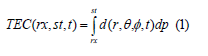
Where:
rx = range or radial position (meters)
st = latitude (degrees)
t = time (seconds)

The TEC computed in (1) is the slant TEC (STEC), which is preferred for this study. It provides a realistic estimation of the variations in the number of electrons per unit of surface along the slant-line path [3]. This slant TEC includes many errors from the original measurements typically classified as Differential Code Bias (DCB) and propagation errors: slight changes in satellite orbit, delays due to interaction with species in the ionosphere and troposphere, timing errors due to inaccurate timing clocks, timing errors due to temperature variation, etc. To be valid, STEC must be corrected for the measurement biases to find Unbiased TEC (UTEC). UTEC can be estimated using GPS pseudo-range measurement along with an estimate of the DCB and propagation errors. The differential pseudo-range can be modeled as in (2) [3].

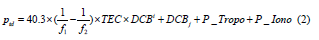
Where:
P__td= The differential pseudo-range measurement
f_₁,f_₂= The GPS measurement frequencies
TEC = The total electron content
DCBi= The ith satellite bias
DCBj= The jth receiver bias
P_Tropo = The tropospheric delay
P_Iono = The ionospheric delay
The UTEC can then be calculated from (2) as

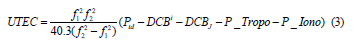
The GPS/GNSS TEC data was obtained from Receiver Independent Exchange format (RINEX) data files from the University NAVSTAR Consortium (UNAVCO), a non-profit organization formed under the auspices of the Cooperative Institute for Research in Environmental Sciences (CIRES) at the University of Colorado Boulder. Differential code biases used in (3) were computed using the techniques developed by Jin [6].

Adaptively truncated hotelling’s T2 test

Of interest in this study is whether real time TEC data are statistically the same from day to day when compared to a baseline TEC (considered to be a non-seismic reference). More specifically, we wish to compare the TEC for several days leading up to seismic activity to that of a known non-seismic baseline. A widely accepted test for this sort of multivariate hypothesis testing is a two-sample Hotelling’s T2 test, which tests the null hypothesis H0:μ1=μ2 where μi is an n-dimensional vector [7]. The T2 test can be computed as

where n1 and n2 are the number of observations in each of the two samples, y₁ and y₂ are the vectorized sample means, and is the pooled sample covariance matrix [7]. For each active GPS receiver, the UTEC computation as described in section 2.1, is performed for each of the 32 operational satellites, sampling once every thirty seconds (twice a minute). This data can be compiled into a 2880×32 matrix, where each column represents a time series of one satellite’s measurements over a given 24- hour period as observed from one ground receiver station. These matrices can then be averaged row-wise to create a single 2880×1 time series vector representing the average TEC at that receiver. Multiple receiver time series are then compiled into a single 2880 by n matrix, where n is the number of receivers for which we have data. This data matrix can be modeled as a random variable of dimension 2880 with n observations per dimension, leading to the formulation of the problem as a multivariate hypothesis test. Since UTEC is functional data, the methods proposed by [7] for adaptive truncation of the Hotelling’s T2 test apply. The test statistic in (4) then becomes:

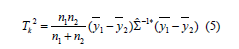
where Σˆ ^−1∗ is now the truncated Moore-Penrose pseudoinverse of the pooled sample covariance matrix [7]. For the truncation of the pseudo-inverse, the methodology as presented in [7] keeps only the p0 greatest eigenvalues and their associated eigenvectors, where p0 is given by:

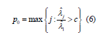
for some threshold, c, which was chosen as c=10-15) for this study. We compute the t-statistic in (5) several times, maintaining k eigenvalues and eigenvectors each time over k=1,…,p0. The maximum t-statistic over the iterations is taken as the statistic value (Figure 1).

Figure 1: Cartoon displaying the GPS receiver geometry and workflow for creating the daily 2880xnTEC matrix for the region, as described in section 2.2.

Figure 2: Plots of the two baselines utilized for this study. On the left is the July 1, 2014 baseline and on the right is the baseline constructed of the pointwise average of TEC in Jan, Feb, and March of 2014.

Figure 3:A map of the napa region in California, USA with markers displaying the locations of the four selected GPS receiver stations (blue) and the epicenter of the August 24 earthquake (red).

Utilizing the adaptively truncated Hotelling’s T2 test, average TEC matrices were tested against each of the baselines. Each day approaching the earthquake was compared to the baselines, beginning on January 1, 2014, and ending on December 30, 2014. For the July 1, 2014 baseline, a graph of the p-values from a selected time range of the tests, July 1 to September 30, is displayed in (Figure 4). Under seismically quiet times, the p-values exhibit a high standard deviation with no discernible daily pattern. Most days under these conditions show a failure to reject the null hypothesis, indicating that they are statistically similar to the non-seismic baseline. During the same time period, there are certain days where the p-values drop to a statistically significant level. However, these drops are not sustained and occur only for a few days before returning to insignificant p-levels. Approaching the date of the earthquake, a considerable, sustained reduction in p-value to significant levels can be observed on July 14 and, other than two outlier spikes on July 31 and August 3, persists until September 9. This behavior in the p-values indicates that TEC becomes consistently uncommon for a significant period before and after the earthquake.

To ensure that the kind of persistent drop in p-value observed in (Figure 4) is not a common behavior, the same test was performed for the two years before the earthquake, 2012 and 2013, and one year after the earthquake, 2015, as shown in (Figure 5). Each of these three years displays behaviors similar to the quiet seismic times in 2014, with no instances of sustained low p-values over a significant period. This behavior suggests that the drop in p-values and its subsequent stabilization over a sustained period is unique to seismically affected times. For the three-month average baseline, a graph of the t-statistic values from the entire year is displayed in (Figure 6). Under seismically quiet times, the t-statistics exhibit consistently low behaviors, fluctuating approximately around a nominal value of 10. During these same time periods, there are certain days that spike to higher values; however, these spikes never exceed a value of 100 and are not sustained for more than one to two days. Beginning at approximately June 1, a slow rise in t-statistic value is exhibited, growing past the date of the earthquake on August 24 and peaking four days after the earthquake on August 28. The t-statistic values begin to descend, returning to their normal non-seismic behavior by approximately September 26. This behavior indicates that TEC has increasingly significant anomalies approaching the time of the earthquake on August 24. To ensure that this kind of rise in t-statistic is not a common behavior, the same test was repeated for the two surrounding years, 2013 and 2015, as shown in (Figure 7). Both surrounding years exhibit behavior similar to 2014 during its quiet seismic times, with no instances of rising behavior in t-values. The results suggest once again that this behavior of the t-values is unique to seismically affected times.

Figure 4:P-values plotted against day of year from the Hotelling’s T2 comparison of the July 1, 2014 baseline to days leading up to and following the August 24 earthquake. A large drop in p-value can be observed on July 14 and persisting until September 9, indicating statistically significant anomalies in TEC prior to the seismic activity.

Figure 5:P-values for Hotelling’s T2 test plotted against day of year for two years prior to the earthquake and one year after the earthquake. The large drop and stabilization exhibited during the year of the earthquake, 2014, does not present in any of the other years, indicating that it is behavior unique to seismically affected times.

Figure 6:T-statistic values plotted against day of year from the Hotelling’s T2 comparison of the three-month average baseline to days leading up to and following the August 24 earthquake. A slow rise in t-statistic can be observed beginning approximately June 1, peaking four days after the earthquake on August 28, and returning to normal behavior on approximately September 26. This indicates increasingly significant anomalies in TEC approaching the earthquake.

Figure 7:T-statistic values for Hotelling’s T2 test plotted against day of year for two years, 2013 and 2015, surrounding the year of the earthquake. The slow rise in t-statistic exhibited during the year of the earthquake, 2014, does not present in any of the other years, indicating that it is behavior unique to seismically affected times.

Previous studies have proposed that measurable anomalies in ionospheric TEC are caused by large-scale seismic activity [1-3]. In this investigation, we utilized adaptively truncated Hotelling’s T2 test to compare the average UTEC for each day to two known baseline signals, July 1 2014 and a pointwise average of each day in the first three months of 2014. Each of these baselines was chosen to approximate a standard background seismic activity in the region under study. Each day, beginning with January 1 and ending with December 30, was compared to each of the baselines using adaptively truncated Hotelling’s T2 test. The resultant t-statistic values and p-values were analyzed to determine if any statistically significant deviations or anomalies exist. For the July 1, 2014 baseline, it was shown that p-values exhibit a high standard deviation under quiet seismic times with no discernible pattern day to day. Approaching the earthquake, there was a sudden drop in p-value on July 14, 2014.

This drop was sustained at the low value past the date of the earthquake on August 24 until it rose and resumed its normal behavior on September 9. The same test was performed on 2012, 2013, and 2015 data showed that a sustained drop in p-value was not exhibited in these years. This indicates that there are statistically significant anomalies in TEC that manifest in the weeks before large seismic activity and that these anomalies are unique to seismic times. For the three-month average baseline, it was shown that under quiet seismic times, t-statistic values exhibit a reasonably consistent behavior, fluctuating around a low nominal value, which in the case of 2014 was approximately 10. Approaching the earthquake, at approximately June 1, a slow rise in t-statistic value can be seen, growing past the earthquake on August 24, peaking four days after the earthquake on August 28, and returning to its normal behavior by approximately September 26. The same test was performed on data from 2013 and 2015, with no instance of this rising behavior in either year. This behavior indicates that increasingly significant anomalies in TEC appear during the weeks approaching significant seismic activity and that these anomalies are unique to seismic times.

In this study, we have shown that anomalies in TEC appear in the weeks approaching large seismic activity compared to both baselines utilized. In addition, these anomalies were shown to be statistically significant (p=0.05). With further research, it may be possible to use such anomalies as part of an earthquake forecasting model which would warn of significant seismic events ahead of time. This study had certain limitations. It does not account for other environmental factors that could potentially influence UTEC. Further work should attempt to account for such environmental factors before performing comparisons. Assumptions on what criteria define approximately regular background seismic activity were also a limiting factor in this study and should be examined in future studies. Additional work should include studies of the “fusion” of the TEC with other earthquake precursors. By analyzing and incorporating multiple precursors in an earthquake forecasting model, the chances of a false positive prediction due to anomalies caused by different mechanisms besides seismic activity can be decreased..

1. Hammerstrom J, Cornely PR (2016) Total Electron Content (TEC) variations and correlation with seismic activity over Japan. Journal of Young Investigators 32(4): 36-40.
2. O Brien M, Cornely PR (2015) Analyzing anomalies in the ionosphere above haiti surrounding the 2010 earthquake. Journal of Young Investigators 29(5): 13-16.
3. Cornely PR, Hughes J (2018) Unbiased Total Electron Content (UTEC), their fluctuations and Correlation with Seismic Activity over Japan. Acta Geophysica 66(1): 51-70.
4. Freund F (2002) Charge generation and propagation in igneous rocks. Journal of Geodynamics 33(5): 545-570.
5. Freund F, Takeuchi A, Lau B (2006) Electric currents streaming out of stressed igneous rock-A step towards understanding pre-earthquake low frequency EM emissions. Physics and Chemistry of Earth 31(9): 389-396.
6. Jin R, Jin S, Feng G (2012) M_DCB: Matlab code for estimating GNSS satellite and receiver differential code biases. GPS Solutions 16: 541-548.
7. Lee J, Cox D, Follen M (2015) A two sample test for functional data. Communications for Statistical Applications and Methods 22(2): 212-135.