Mathematical Modeling and Analysis of Leukaemia Transmission: Homotopy Perturbation Method

Leukaemia is a broad term for cancers of the blood cells. The type of Leukaemia depends on the type of blood cell that becomes cancer and whether it grows quickly or slowly. There are several types of Leukaemia, which are divided based mainly on whether the Leukaemia is acute (fast-growing) or chronic (slower growing) and whether it starts in myeloid cells or lymphoid cells [1]. Leukaemia occurs most often in adults older than 55, but it is also the most common cancer in children younger than 15. Explore the links on this page to learn more about the types of Leukaemia plus treatment, statistics, research, and clinical trials. NCI does not have any evidence-based information about the prevention of Leukaemia [2,3].

Leukaemia is grouped in two ways: the type of white blood cell affected - lymphoid or myeloid; and how quickly the disease develops and worsens. Acute leukaemia appears suddenly and multiplies, while chronic leukaemia appears gradually and develops slowly over months to years. This information refers to four types of leukaemia; acute lymphoblastic leukaemia, chronic lymphocytic leukaemia, acute myeloid leukaemia and chronic myeloid leukaemia. The cause of acute leukaemia is unknown, but factors that put some people at higher risk are:

A. Exposure to intense radiation.

B. Exposure to certain chemicals, such as benzene.

C. Certain viral infections (Viruses like the Human T-cell/ leukaemia virus)

D. Certain genetic syndromes.

The Philadelphia chromosome is defective in most persons diagnosed with chronic myeloid Leukaemia. It has also been related to high levels of radiation exposure [4]. In addition, certain irregularities in the blood cause the cell to grow hastily, and these abnormal cells rule healthy blood cells in the bone marrow. Consequently, the three types of blood cells (white blood cells/T cells, red blood cells, and platelets) gradually die out from the blood Leukemia disease doesn’t cure entirely because of its setbacks in the blood. Despite this, it is indispensable to control this distressing disease, Leukaemia and Khatun et al. [5] purpose, optimal control theory to discuss the optimization of Leukaemia.

Optimal control theory is an influential mathematical tool used to make decisions involving critical biological situations. It is often used to control the spread of most diseases [6-7]. Many of the researchers investigated about Optimal control theory for various diseases. For example, Moore and Li used a simple mathematical model to study the dynamics of chronic myelogenous leukaemia [8]. Nowak et al. [9] suggested a rigorous mathematical study of cancer immunotherapy. Blaineh et al. [10] presented an optimal control investigation of the dynamics of a vector-transmitted disease using two deterministic models. Eryn et al. [11] and the national cancer institute [12] developed a simple mathematical model of Leukaemia to study the dynamics of it and then apply optimal control theory to analyse the optimal strategy of the treatment of Leukaemia using immune-boosting drugs and adoptive T cell therapy.

In this paper, the mathematical model of Leukaemia is discussed. The model has non-linear equations which represent rates of change for susceptible cells, infected cells as well as immune cells. We used the Homotopy Perturbation Method to solve the system of non-linear equations. Recently a modified approach of the Homotopy Perturbation Method has been used to derive an approximate analytical expression for each of the nine different groups that form population in HIV/AIDS transmission dynamics [13].

In this paper, we discuss the model which depicts leukaemia transmission in three compartments. (Figure 1) represents the Flowchart of the model of leukaemia transmission without control. The three compartments are susceptible cells S, infected cells I and immune cells W. In these compartments which are not infected with leukaemia disease but can be infected is defined as susceptible compartment denoted by S. The compartment which is infected with leukaemia and able to transmit leukaemia is defined as infective compartment and denoted by I. Again, recovered individuals are those who are removed from the susceptible-infective interaction by recovery with immunity, isolation by any process is defined as recovered compartment and denoted by W. Further, let A be the rate at which the susceptible blood cells entering into the circulatory blood from compartments like bone marrow, lymph nodes and thymus.

Figure 1: Schematic diagram of the model of leukemia transmission (without optimal control).

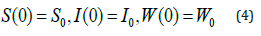
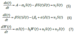
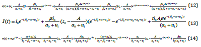
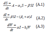
The natural mortality rates of vulnerable blood cells, infected cells, and immune cells are represented by the parameters a0, α0 and b0, respectively. The infection rate of vulnerable blood cells is the metric. The rate at which infected cells recover after contact with immune cells is represented by α. As a result, this resurrected phrase has been added to the immune cells compartment. The equations that govern our model are as follows:

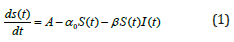
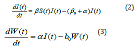
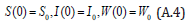
with the initial conditions are

The model with control, which illustrates leukaemia transmission in three compartments, is discussed in this section. We insert two control variables, represented by u, into the dynamics (u1, u2). Leukaemia is caused by two mutations in the cell’s DNA (chromosome translocation and Philadelphia Chromosome). Some risk factors for leukaemia include cigarette smoking, alcohol, drug usage, and blood problems (such as Li-Fraumeni syndrome, Down syndrome, Bloom syndrome, and other medical illnesses). As far as we know, there are no viable vaccines or medications available to cure leukaemia in the blood entirely.

After being infected with leukaemia, the disease can be controlled with I immune-boosting medications or chemotherapy, (ii) adoptive T cell treatment (also known as gene therapy) or immunotherapy, which harness the patient’s immune system’s ability to fight disease. As a result, our control u1(t) is concerned with treating immune-boosting medications, whereas u2(t) is concerned with the immunotherapeutic treatment of leukaemia cure. We depict the flowchart presentation of the compartmental model with the regulation of leukaemia transmission in (Figure 2) using these assumptions. We can reformulate the model (1) of the following using the previous figure.

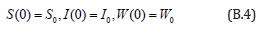
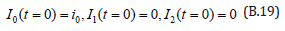
with the initial conditions are

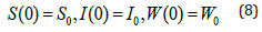
Figure 2: Schematic diagram of the model of leukemia transmission (with control).

It has been found that several analytical or semi analytical methods for solving nonlinear differential equations even with strong nonlinearities have been developed in recent years. Of these methods, we mention Homotopy analysis method [14,15], Adomian decomposition method [16], variational iteration method [17], Green’s function iterative method [18,19], Homotopy Perturbation Method (HPM) [20-22] and Agbariganji Method [23-26] the has received great deal of attention [27-30].

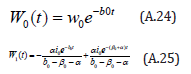
By solving Eqs. (1)-(4) using the Homotopy Perturbation Method (Appendix A) we obtain the solution as follows:

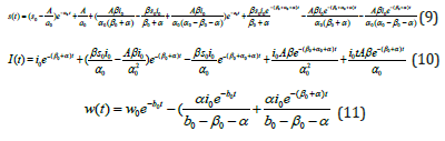
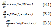
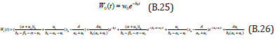
By solving Eqs. (5)-(8) using the Homotopy Perturbation Method (Appendix B) we obtain the solution as follows:

We execute numerical simulations of leukaemia transmission model (1)-(4) and optimal control model (5)-(8) and for which we use a set of logical parameter values. The simulation is performed using ODE45 solver written in MATLAB programming. Eqns. (9)- (12) and Eqns. (13)-(15) are very closed expressions for the models Eqns. (1)-(4) and Eqns.(5)-(8). We compared our analytical solutions obtained by HPM with the numerical simulation obtained by MATLAB software. To test the accuracy of our approximate analytical expressions, the system (1)-(4) and (5)-(8) are also solved by numerically by using MATLAB for all possible values of parameters. The MATLAB program is also given in Appendix C (Figure 3).

Figure 3: Comparison of our analytical expression of SIW with the numerical result for the various values of the parameters using leukemia without control.

In treating the Leukaemia model without control, equations (9) to (11) represent the analytical expression for the susceptible blood cells, infected cells, and Immune cells. Equations (12) to (14) provide the analytical expression for the susceptible blood cells, Infected cells, and Immune cells in the Leukaemia model with control.

(Figure 4) and (Figure 5) represents the change in susceptible blood cells and infected cells over 50 days for various infection rates or interaction rates with cancer cells in the patient’s body. For decreasing levels of β, one can see that the number of susceptible blood cells increases. It indicates that as the infection rate rises, the number of susceptible blood cells decreases. This is due to the fact that susceptible blood cells are drawn to infected cells in order to interact with cancer cells in the body.

Figure 4: The rate of Susceptible cells for various values of α0 and β (Leukemia without control).

Figure 5: The rate of infected cells for various values of α, α0, β and β0 (Leukemia without control).

Different phenomena can be observed in infected cells. As the number of infected cells in the blood increases, so does the number of cancer cells infect. It means that when cancer cells interact with susceptible cells, infected cells are produced, and the concentration of infected cells rises substantially as the interaction rate in the blood circulatory system rises. In addition, (Figure 6) depicts the variation of immune cells for various values of β. The number of immune cells grows as the infection rate in the patient’s blood decreases, as seen in (Figure 6). This means that cancer cells interact with immune cells at a lower rate. In normal, human immune cells, also known as T cells, attack infection in the body; but, when infection rates rise, the immune system weakens, and immune cells cannot operate normally.

Figure 6: The rate of infected cells for various values of α and b0 leukemia without control.

(Figure 7) indicates the variation of susceptible, infected, and immune cells during 50 days with fixed values for other parameters. Moreover, in Figure 7(A), when u1=0, u2=0.01, and in Figure 7(B), when u1=0.01, u2=0, we compared all three cells and the function of susceptible blood cells and infected cells is rising, whilst the function of immune cells is decreasing. It can be seen in the diagram that the susceptible blood cells are soaring towards higher recovery rates (Table 1).

Figure 6: The rate of infected cells for various values of α and b0 leukemia without control.

(Figure 7) indicates the variation of susceptible, infected, and immune cells during 50 days with fixed values for other parameters. Moreover, in Figure 7(A), when u1=0, u2=0.01, and in Figure 7(B), when u1=0.01, u2=0, we compared all three cells and the function of susceptible blood cells and infected cells is rising, whilst the function of immune cells is decreasing. It can be seen in the diagram that the susceptible blood cells are soaring towards higher recovery rates (Table 1).

Figure 7: Rate of SIW for the various values of the parameter u1 and u2 leukemia with control.

Table 1: Susceptible blood cells, Infected cells, Immune cells. (Nomenclature and Units).

We discuss the SIR (Susceptible - Infected - Recovered) model of Leukaemia with two cases in this work. Both models are solved using the Homotopy Perturbation Method, and numerical simulations demonstrate the analytic results. We see that the rate of infected cells and immune cells significantly impacts the disease’s spread. Immunotherapy is now considered to be the most promising cancer treatment. When the number of infected cells rises, the number of immune cells in the body falls. On the other hand, immunotherapy and immune-boosting medicines increase the number of immune cells in a patient. Our study revealed that a combination of the two would be the most effective method to control this disease.

Appendix A: Analytical solution on nonlinear Eqns. (1)- (4) using Homotopy Perturbation Method (HPM).

with the initial conditions are

The Homotopy form the Eqns. (A.1) -(A.4) can be constructed as follows:

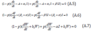
where p is the embedding parameter and p∈[0,1] , The approximate solution of (A.5) to (A.7) are

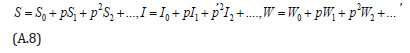
Substituting Eqns. (A.8) into (A.5) -(A.7), gives the following result.

Comparing the coefficients of like powers of p in Eqn. (A.8) gives:

The initial conditions are,

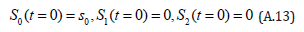
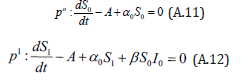
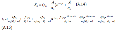
The solution of the Eqns. (A.11) and (A.12) are given by

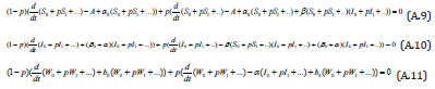
Comparing the coefficients of like powers of p in Eqn. (A.9) gives:

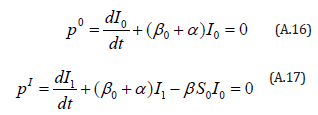
The initial conditions are,

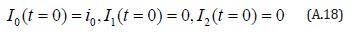
The solution of the Eqns. (A.16) and (A.17) are given by

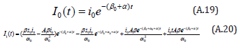
Comparing the coefficients of like powers of p in Eqn. (A.10) gives:

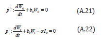
The initial conditions are,

The solution of the Eqns. (A.21) and (A.22) are given by

Appendix B: Analytical solution on nonlinear Eqns. (5)- (8) using Homotopy Perturbation Method (HPM).

Consider the differential equation

with the initial conditions are

The Homotopy form the Eqns. (B.1) -(B.3) can be constructed as follows:

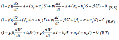
where is the embedding parameter and p∈[0,1] , The approximate solution of (B.5) to (B.7) are

Substituting Eqns. (B.8) into (B.5) - (B.7), gives the following result.

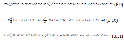
Comparing the coefficients of like powers of p in Eqn. (B.9) gives:

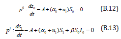
The initial conditions are,

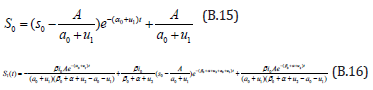
The solution of the Eqns. (B.12) & (B.13) are given by

Comparing the coefficients of like powers of p in Eqn. (B.10) gives:

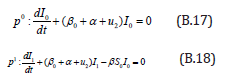
The initial conditions are,

The solution of the Eqns. (B.17) and (B.18) are given by

Comparing the coefficients of like powers of p in Eqn. (B.11) gives:

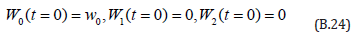
The initial conditions are,

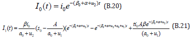
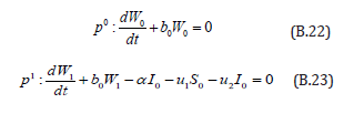
The solution of the Eqns. (B.22) & (B.23) are given by

1. Leukemia- American Cancer Society.
2. Khatun MS, Biswas MHA (2020) Mathematical analysis and optimal control applied to the treatment of leukemia. Journal of Applied Mathematics and Computing 64(1-2): 331-353.
3. Leukemia-Patient Version - National Cancer Institute.
4. Leukaemia, Causes, Symptoms & Treatments. Cancer Council, Australia.
5. Mayo Clinic Family Health Book. (5^th edn), Diseases-conditions, Leukemia, Symptoms-causes, syc-20374373.
6. Khatun MS, Biswas MHA (2020) Optimal control strategies for preventing hepatitis B infection and reducing chronic liver cirrhosis incidence. Infect Dis Model 5: 91-110.
7. Swan GW (1990) Role of optimal control theory in cancer chemotherapy. Math Biosci 101(2): 237-284.
8. Moore H, Li NK (2004) A mathematical model of chronic myelogenous leukemia (CML) and T interaction. J Theor Biol 227(4): 513-523.
9. Nowak M, May RM (2000) Virus dynamics: Mathematical principles of immunology and virology. Oxford University Press, UK.
10. Blayneh, K, Cao Y, Kwon HD (2009) Optimal control of vector-borne diseases: Treatment and prevention. Discrete And Continuous Dynamical Systems Series B 11 (3): 587-611.
11. Eryn B (2011) Huge results raise hope for cancer breakthrough. Los Angeles Times, USA.
12. (2017) CAR T cells: Engineering patients’ immune cells to treat their cancers. National Cancer Institute.
13. Shanta Khatun, Haider Ali Biswas (2020) Mathematical analysis and optimal control applied to the treatment of leukemia. Journal of Applied Mathematics and Computing 64: 331-353.
14. Saravanakumar K, Rajendran L (2015) Mathematical analysis of an enzyme-entrapped conducting polymer modified electrode. Appl Math Model 39: 7351-7363.
15. Jafari H, Seifi S (2009) Homotopy analysis method for solving linear and nonlinear fractional diffusion-wave equation. Commun. Nonlinear Sci 14(5): 2006-2012.
16. Abukhaled M (2013) Variational iteration method for nonlinear singular two-point boundary value problems arising in human physiology. J Math 2: 1-4.
17. Wazwaz AMA (1999) Reliable modification of adomian decomposition method. Appl Math Comput 102(1): 77-86.
18. Abukhaled M, Khuri SA (2017) A semi-analytical solution of amperometric enzymatic reactions based on green’s functions and fixed point iterative schemes. J Electroanal Chem 792: 66-71.
19. Abukhaled M (2017) Green’s function iterative approach for solving strongly nonlinear oscillators. J Comput Nonlinear Dyn 12(5): 051021.
20. He JH (1999) Homotopy perturbation technique. Appl Mech Eng 178(3-4): 257-262.
21. He JH (2014) Homotopy perturbation method with two expanding parameters. Indian J Phys 88:193-196.
22. Swaminathan R, Lakshmi Narayanan K, Mohan V, Saranya K, Rajendran L (2019) Reaction/diffusion equation with michaelis-menten kinetics in microdisk biosensor: Homotopy perturbation method approach. Int J Electrochem Sci 14: 3777-3791.
23. Akbari MR, Ganji DD, Majidian A, Ahmadi AR (2014) Solving nonlinear differential equations of Vanderpol, Rayleigh and Duffing by AGM. Front Mech Eng 9: 177-190.
24. Akbari MR, Ganji DD, Goltabar AR (2014) Dynamics vibration analysis for nonlinear partial differential equation of the beam-columns with shear deformation and rotary inertia by AGM. Dev Appl Ocean Eng (DAOE) 3: 22-23.
25. Dharmalingam KM, Veeramuni M (2019) Akbari-Ganji’s Method (AGM) for solving non-linear reaction - Diffusion equation in the electroactive polymer film. J Electroanal Chem 844:1-5.
26. Visuvasam J, Meena, A, Rajendran L (2020) New analytical method for solving nonlinear equation in rotating disk electrodes for second order ECE reactions. Journal of Electroanalytical Chemistry 869:114106.
27. Rodrigues DS, Mancera PFA, Carvalhoc T, Gonçalves LF (2019) A mathematical model for chemoimmunotherapy of chronic lymphocytic leukaemia. Journal of Applied Mathematics and Computation 349: 118-133.
28. Nani F, Freedman HI (2000) A mathematical model of cancer treatment by immunotherapy. Mathematical Biosciences 163(2): 159-199.
29. Moore H, Li NK (2004) A mathematical model for Chronic Myelogenous Leukemia (CML) and T cell interaction. J Theor Biol 227(4): 513-523.
30. Saravanakumar S, Eswari, Abukhaled M, Rajendran L (2000) A mathematical model of risk factors in HIV/AIDS transmission dynamics: observational study of female sexual network in India. Applied Mathematics & Information Sciences 14(6): 196-976.